WRDS, CRSP, and Compustat

Note

You are reading Tidy Finance with Python. You can find the equivalent chapter for the sibling Tidy Finance with R here.

This chapter shows how to connect to Wharton Research Data Services (WRDS), a popular provider of financial and economic data for research applications. We use this connection to download the most commonly used data for stock and firm characteristics, CRSP and Compustat. Unfortunately, this data is not freely available, but most students and researchers typically have access to WRDS through their university libraries. Assuming that you have access to WRDS, we show you how to prepare and merge the databases and store them in the SQLite database introduced in the previous chapter. We conclude this chapter by providing some tips for working with the WRDS database.

If you don’t have access to WRDS but still want to run the code in this book, we refer to WRDS Dummy Data, where we show how to create a dummy database that contains the WRDS tables and corresponding columns. With this database at hand, all code chunks in this book can be executed with this dummy database.

First, we load the Python packages that we use throughout this chapter. Later on, we load more packages in the sections where we need them. The last two packages are used for plotting.

import pandas as pd
import numpy as np
import tidyfinance as tf
import sqlite3

from plotnine import *
from mizani.formatters import comma_format, percent_format
from datetime import datetime

We use the same date range as in the previous chapter to ensure consistency. However, we have to use the date format that the WRDS database expects.

start_date = "01/01/1960"
end_date = "12/31/2023"

Accessing WRDS

WRDS is the most widely used source for asset and firm-specific financial data used in academic settings. WRDS is a data platform that provides data validation, flexible delivery options, and access to many different data sources. The data at WRDS is also organized in an SQL database, although they use the PostgreSQL engine. This database engine is just as easy to handle with Python as SQL. We use the sqlalchemy package to establish a connection to the WRDS database because it already contains a suitable driver.¹

from sqlalchemy import create_engine

To establish a connection to WRDS, you use the function create_engine() with a connection string that specifies the WRDS server and your login credentials. We defined environment variables for the purpose of this book because we obviously do not want (and are not allowed) to share our credentials with the rest of the world. See Setting Up Your Environment for information about why and how to create an .env-file that can be loaded with load_dotenv(). Alternatively, you can replace os.getenv('WRDS_USER) and os.getenv('WRDS_PASSWORD') with your own credentials (but be careful not to share them with others or the public).

Additionally, you have to use two-factor authentication since May 2023 when establishing a remote connection to WRDS. You have two choices to provide the additional identification. First, if you have Duo Push enabled for your WRDS account, you will receive a push notification on your mobile phone when trying to establish a connection with the code below. Upon accepting the notification, you can continue your work. Second, you can log in to a WRDS website that requires two-factor authentication with your username and the same IP address. Once you have successfully identified yourself on the website, your username-IP combination will be remembered for 30 days, and you can comfortably use the remote connection below.

import os
from dotenv import load_dotenv
load_dotenv()

connection_string = (
  "postgresql+psycopg2://"
 f"{os.getenv('WRDS_USER')}:{os.getenv('WRDS_PASSWORD')}"
  "@wrds-pgdata.wharton.upenn.edu:9737/wrds"
)

wrds = create_engine(connection_string, pool_pre_ping=True)

You can also use the tidyfinance package to set the login credentials and create a connection.

tf.set_wrds_credentials()
wrds = tf.get_wrds_connection()

The remote connection to WRDS is very useful. Yet, the database itself contains many different tables. You can check the WRDS homepage to identify the table’s name you are looking for (if you go beyond our exposition).

Downloading and Preparing CRSP

The Center for Research in Security Prices (CRSP) provides the most widely used data for US stocks. We use the wrds engine object that we just created to first access monthly CRSP return data. Actually, we need two tables to get the desired data: (i) the CRSP monthly security file (msf), and (ii) the historical identifying information (stksecurityinfohist).

We use the two remote tables to fetch the data we want to put into our local database. Just as above, the idea is that we let the WRDS database do all the work and just download the data that we actually need. We apply common filters and data selection criteria to narrow down our data of interest: (i) we use only stock prices from NYSE, Amex, and NASDAQ (primaryexch %in% c("N", "A", "Q")) when or after issuance (conditionaltype %in% c("RW", "NW")) for actively traded stocks (tradingstatusflg == "A")², (ii) we keep only data in the time windows of interest, (iii) we keep only US-listed stocks as identified via no special share types (sharetype = 'NS'), security type equity (securitytype = 'EQTY'), security sub type common stock (securitysubtype = 'COM'), issuers that are a corporation (issuertype %in% c("ACOR", "CORP")), and (iv) we keep only months within permno-specific start dates (secinfostartdt) and end dates (secinfoenddt). As of July 2022, there is no need to additionally download delisting information since it is already contained in the most recent version of msf (see our blog post about CRSP 2.0 for more information). Additionally, the industry information in stksecurityinfohist records the historic industry and should be used instead of the one stored under same variable name in msf_v2.

crsp_monthly_query = (
  "SELECT msf.permno, date_trunc('month', msf.mthcaldt)::date AS date, "
         "msf.mthret AS ret, msf.shrout, msf.mthprc AS altprc, "
         "ssih.primaryexch, ssih.siccd "
    "FROM crsp.msf_v2 AS msf "
    "INNER JOIN crsp.stksecurityinfohist AS ssih "
    "ON msf.permno = ssih.permno AND "
       "ssih.secinfostartdt <= msf.mthcaldt AND "
       "msf.mthcaldt <= ssih.secinfoenddt "
   f"WHERE msf.mthcaldt BETWEEN '{start_date}' AND '{end_date}' "
          "AND ssih.sharetype = 'NS' "
          "AND ssih.securitytype = 'EQTY' "  
          "AND ssih.securitysubtype = 'COM' " 
          "AND ssih.usincflg = 'Y' " 
          "AND ssih.issuertype in ('ACOR', 'CORP') " 
          "AND ssih.primaryexch in ('N', 'A', 'Q') "
          "AND ssih.conditionaltype in ('RW', 'NW') "
          "AND ssih.tradingstatusflg = 'A'"
)

crsp_monthly = (pd.read_sql_query(
    sql=crsp_monthly_query,
    con=wrds,
    dtype={"permno": int, "siccd": int},
    parse_dates={"date"})
  .assign(shrout=lambda x: x["shrout"]*1000)
)

Now, we have all the relevant monthly return data in memory and proceed with preparing the data for future analyses. We perform the preparation step at the current stage since we want to avoid executing the same mutations every time we use the data in subsequent chapters.

The first additional variable we create is market capitalization (mktcap), which is the product of the number of outstanding shares (shrout) and the last traded price in a month (prc). Note that in contrast to returns (ret), these two variables are not adjusted ex-post for any corporate actions like stock splits. Therefore, if you want to use a stock’s price, you need to adjust it with a cumulative adjustment factor. We also keep the market cap in millions of USD just for convenience, as we do not want to print huge numbers in our figures and tables. In addition, we set zero market capitalization to missing as it makes conceptually little sense (i.e., the firm would be bankrupt).

crsp_monthly = (crsp_monthly
  .assign(mktcap=lambda x: x["shrout"]*x["altprc"]/1000000)
  .assign(mktcap=lambda x: x["mktcap"].replace(0, np.nan))
)

The next variable we frequently use is the one-month lagged market capitalization. Lagged market capitalization is typically used to compute value-weighted portfolio returns, as we demonstrate in a later chapter. The most simple and consistent way to add a column with lagged market cap values is to add one month to each observation and then join the information to our monthly CRSP data.

mktcap_lag = (crsp_monthly
  .assign(
    date=lambda x: x["date"]+pd.DateOffset(months=1),
    mktcap_lag=lambda x: x["mktcap"]
  )
  .get(["permno", "date", "mktcap_lag"])
)

crsp_monthly = (crsp_monthly
  .merge(mktcap_lag, how="left", on=["permno", "date"])
)

Next, we transform primary listing exchange codes to explicit exchange names.

def assign_exchange(primaryexch):
    if primaryexch == "N":
        return "NYSE"
    elif primaryexch == "A":
        return "AMEX"
    elif primaryexch == "Q":
        return "NASDAQ"
    else:
        return "Other"

crsp_monthly["exchange"] = (crsp_monthly["primaryexch"]
  .apply(assign_exchange)
)

Similarly, we transform industry codes to industry descriptions following Bali, Engle, and Murray (2016). Notice that there are also other categorizations of industries (e.g., Fama and French 1997) that are commonly used.

def assign_industry(siccd):
    if 1 <= siccd <= 999:
        return "Agriculture"
    elif 1000 <= siccd <= 1499:
        return "Mining"
    elif 1500 <= siccd <= 1799:
        return "Construction"
    elif 2000 <= siccd <= 3999:
        return "Manufacturing"
    elif 4000 <= siccd <= 4899:
        return "Transportation"
    elif 4900 <= siccd <= 4999:
        return "Utilities"
    elif 5000 <= siccd <= 5199:
        return "Wholesale"
    elif 5200 <= siccd <= 5999:
        return "Retail"
    elif 6000 <= siccd <= 6799:
        return "Finance"
    elif 7000 <= siccd <= 8999:
        return "Services"
    elif 9000 <= siccd <= 9999:
        return "Public"
    else:
        return "Missing"

crsp_monthly["industry"] = (crsp_monthly["siccd"]
  .apply(assign_industry)
)

Next, we compute excess returns by subtracting the monthly risk-free rate provided by our Fama-French data. As we base all our analyses on the excess returns, we can drop the risk-free rate from our data frame. Note that we ensure excess returns are bounded by -1 from below as a return less than -100% makes no sense conceptually. Before we can adjust the returns, we have to connect to our database and load the data frame factors_ff3_monthly.

tidy_finance = sqlite3.connect(database="data/tidy_finance_python.sqlite")

factors_ff3_monthly = pd.read_sql_query(
  sql="SELECT date, rf FROM factors_ff3_monthly",
  con=tidy_finance,
  parse_dates={"date"}
)
  
crsp_monthly = (crsp_monthly
  .merge(factors_ff3_monthly, how="left", on="date")
  .assign(ret_excess=lambda x: x["ret"]-x["rf"])
  .assign(ret_excess=lambda x: x["ret_excess"].clip(lower=-1))
  .drop(columns=["rf"])
)

The tidyfinance package provides a shortcut to implement all these processing steps from above:

crsp_monthly = tf.download_data(
  domain="wrds",
  dataset="crsp_monthly",
  start_date=start_date,
  end_date=end_date
)

Since excess returns and market capitalization are crucial for all our analyses, we can safely exclude all observations with missing returns or market capitalization.

crsp_monthly = (crsp_monthly
  .dropna(subset=["ret_excess", "mktcap", "mktcap_lag"])
)

Finally, we store the monthly CRSP file in our database.

(crsp_monthly
  .to_sql(name="crsp_monthly", 
          con=tidy_finance, 
          if_exists="replace",
          index=False)
)

First Glimpse of the CRSP Sample

Before we move on to other data sources, let us look at some descriptive statistics of the CRSP sample, which is our main source for stock returns.

Figure 1 shows the monthly number of securities by listing exchange over time. NYSE has the longest history in the data, but NASDAQ lists a considerably large number of stocks. The number of stocks listed on AMEX decreased steadily over the last couple of decades. By the end of {python} crsp_monthly['date'].max().year, there were {python} len(crsp_monthly.loc[(crsp_monthly['date'] == crsp_monthly['date'].max()) & (crsp_monthly['exchange'] == 'NASDAQ'), 'permno'].unique()) stocks with a primary listing on NASDAQ, {python} len(crsp_monthly.loc[(crsp_monthly['date'] == crsp_monthly['date'].max()) & (crsp_monthly['exchange'] == 'NYSE'), 'permno'].unique()) on NYSE, and {python} len(crsp_monthly.loc[(crsp_monthly['date'] == crsp_monthly['date'].max()) & (crsp_monthly['exchange'] == 'AMEX'), 'permno'].unique()) on AMEX.

securities_per_exchange = (crsp_monthly
  .groupby(["exchange", "date"])
  .size()
  .reset_index(name="n")
)

securities_per_exchange_figure = (
  ggplot(
    securities_per_exchange, 
    aes(x="date", y="n", color="exchange", linetype="exchange")
  )
  + geom_line()
  + labs(
      x="", y="", color="", linetype="",
      title="Monthly number of securities by listing exchange"
    )
  + scale_x_datetime(date_breaks="10 years", date_labels="%Y")
  + scale_y_continuous(labels=comma_format())
)
securities_per_exchange_figure.show()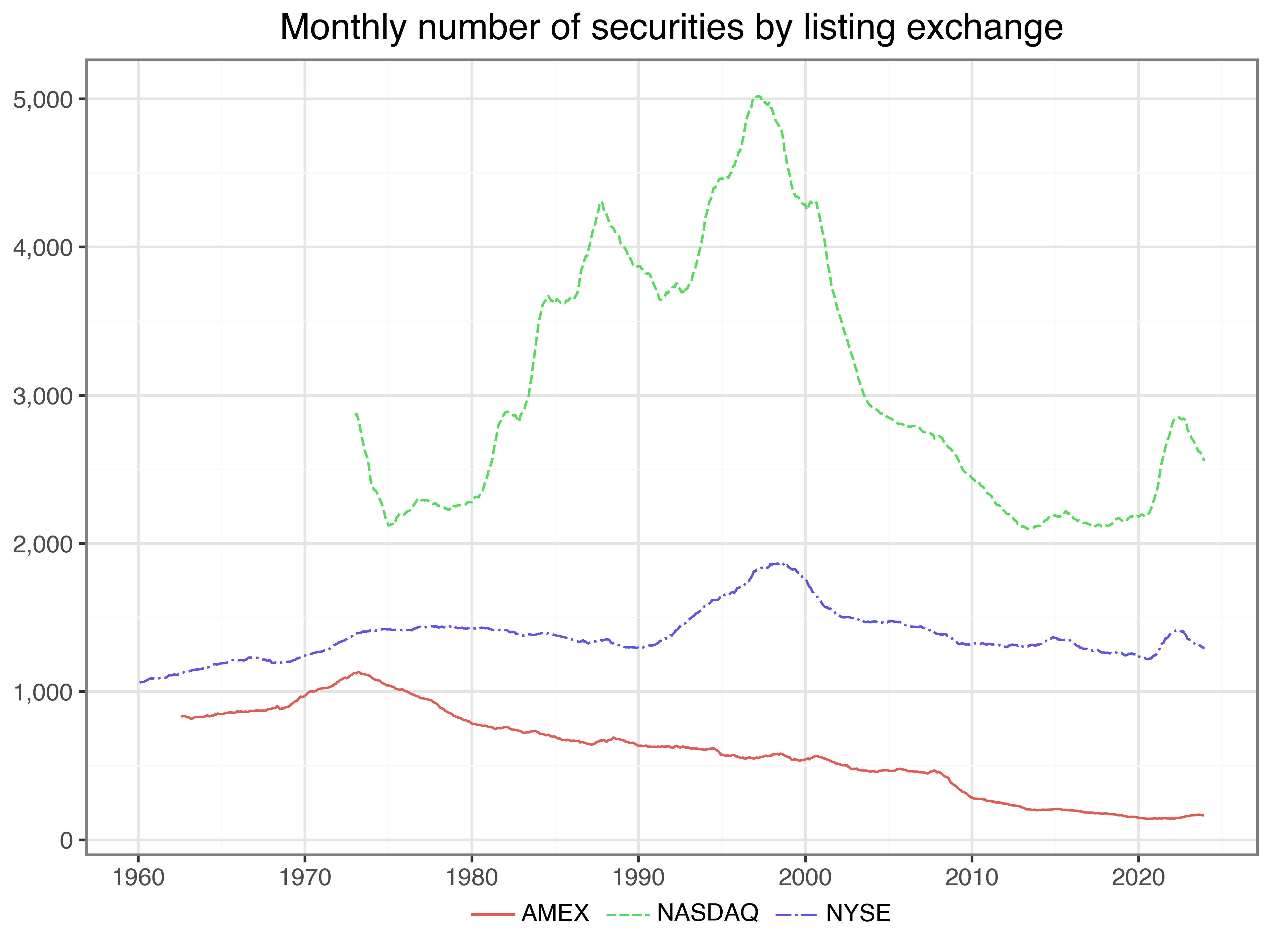

Figure 1: The figure shows the monthly number of stocks in the CRSP sample listed at each of the US exchanges.

Next, we look at the aggregate market capitalization grouped by the respective listing exchanges in Figure 2. To ensure that we look at meaningful data that is comparable over time, we adjust the nominal values for inflation. In fact, we can use the tables that are already in our database to calculate aggregate market caps by listing exchange. All values in Figure 2 are in terms of the end of 2023 USD to ensure intertemporal comparability. NYSE-listed stocks have by far the largest market capitalization, followed by NASDAQ-listed stocks.

cpi_monthly = pd.read_sql_query(
  sql="SELECT * FROM cpi_monthly",
  con=tidy_finance,
  parse_dates={"date"}
)

market_cap_per_exchange = (crsp_monthly
  .merge(cpi_monthly, how="left", on="date")
  .groupby(["date", "exchange"])
  .apply(
    lambda group: pd.Series({
      "mktcap": group["mktcap"].sum()/group["cpi"].mean()
    })
  )
  .reset_index()
)

market_cap_per_exchange_figure = (
  ggplot(
    market_cap_per_exchange, 
    aes(x="date", y="mktcap/1000", color="exchange", linetype="exchange")
  )
  + geom_line()
  + labs(
      x="", y="", color="", linetype="",
      title="Monthly market cap by listing exchange in billions of Dec 2023 USD"
    )
  + scale_x_datetime(date_breaks="10 years", date_labels="%Y")
  + scale_y_continuous(labels=comma_format())
)
market_cap_per_exchange_figure.show()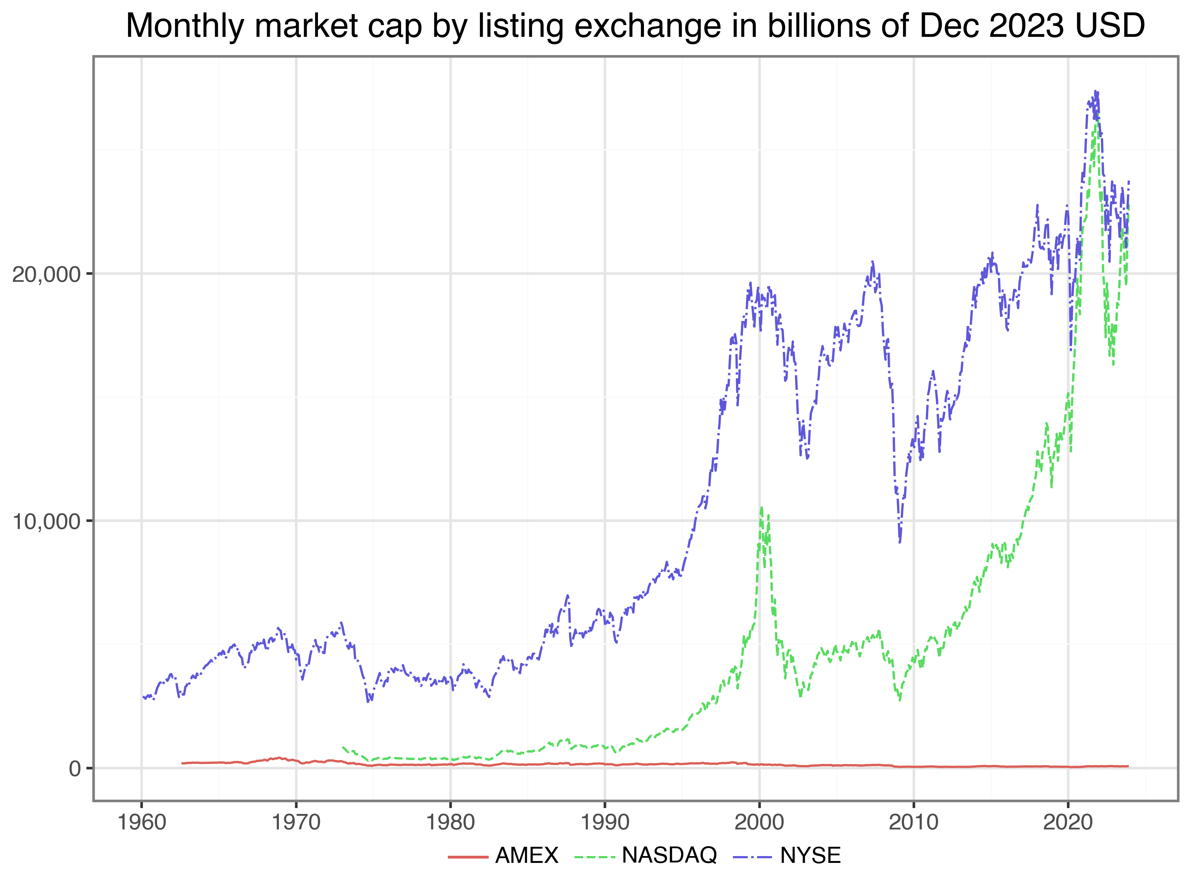

Figure 2: The figure shows the monthly market capitalization by listing exchange. Market capitalization is measured in billion USD, adjusted for consumer price index changes such that the values on the horizontal axis reflect the buying power of billion USD in December 2023.

Next, we look at the same descriptive statistics by industry. Figure 3 plots the number of stocks in the sample for each of the SIC industry classifiers. For most of the sample period, the largest share of stocks is in manufacturing, albeit the number peaked somewhere in the 90s. The number of firms associated with public administration seems to be the only category on the rise in recent years, even surpassing manufacturing at the end of our sample period.

securities_per_industry = (crsp_monthly
  .groupby(["industry", "date"])
  .size()
  .reset_index(name="n")
)

linetypes = ["-", "--", "-.", ":"]
n_industries = securities_per_industry["industry"].nunique()

securities_per_industry_figure = (
  ggplot(
    securities_per_industry, 
    aes(x="date", y="n", color="industry", linetype="industry")
  )
  + geom_line()
  + labs(
      x="", y="", color="", linetype="",
      title="Monthly number of securities by industry"
    )
  + scale_x_datetime(date_breaks="10 years", date_labels="%Y")
  + scale_y_continuous(labels=comma_format())
  + scale_linetype_manual(
      values=[linetypes[l % len(linetypes)] for l in range(n_industries)]
    ) 
)
securities_per_industry_figure.show()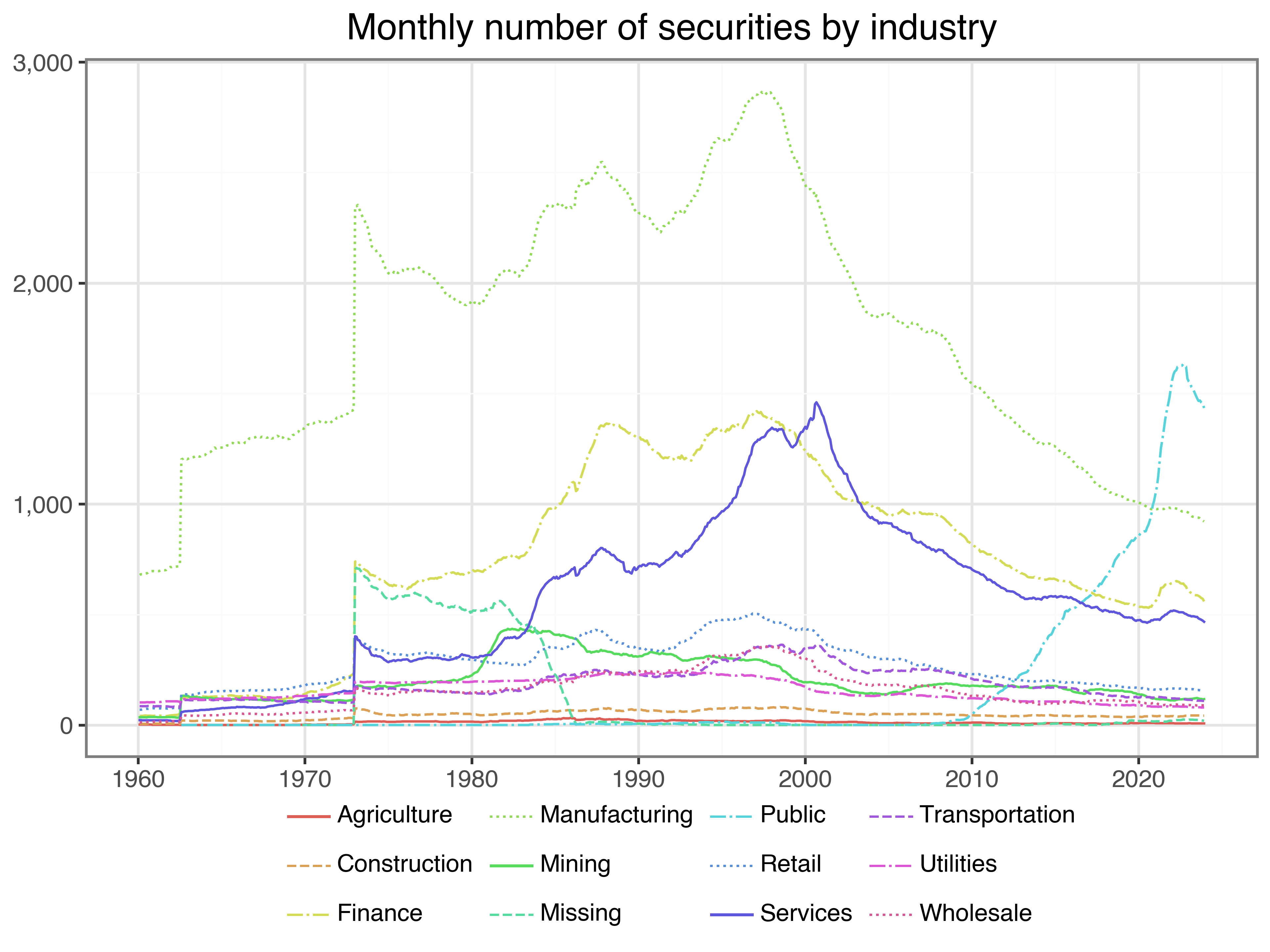

Figure 3: The figure shows the monthly number of stocks in the CRSP sample associated with different industries.

We also compute the market cap of all stocks belonging to the respective industries and show the evolution over time in Figure 4. All values are again in terms of billions of end of 2023 USD. At all points in time, manufacturing firms comprise of the largest portion of market capitalization. Toward the end of the sample, however, financial firms and services begin to make up a substantial portion of the market cap.

market_cap_per_industry = (crsp_monthly
  .merge(cpi_monthly, how="left", on="date")
  .groupby(["date", "industry"])
  .apply(
    lambda group: pd.Series({
      "mktcap": (group["mktcap"].sum()/group["cpi"].mean())
    })
  )
  .reset_index()
)

market_cap_per_industry_figure = (
  ggplot(
    market_cap_per_industry, 
    aes(x="date", y="mktcap/1000", color="industry", linetype="industry")
  )
  + geom_line()
  + labs(
      x="", y="", color="", linetype="",
      title="Monthly market cap by industry in billions of Dec 2023 USD"
    )
  + scale_x_datetime(date_breaks="10 years", date_labels="%Y")
  + scale_y_continuous(labels=comma_format())
  + scale_linetype_manual(
      values=[linetypes[l % len(linetypes)] for l in range(n_industries)]
    ) 
)
market_cap_per_industry_figure.show()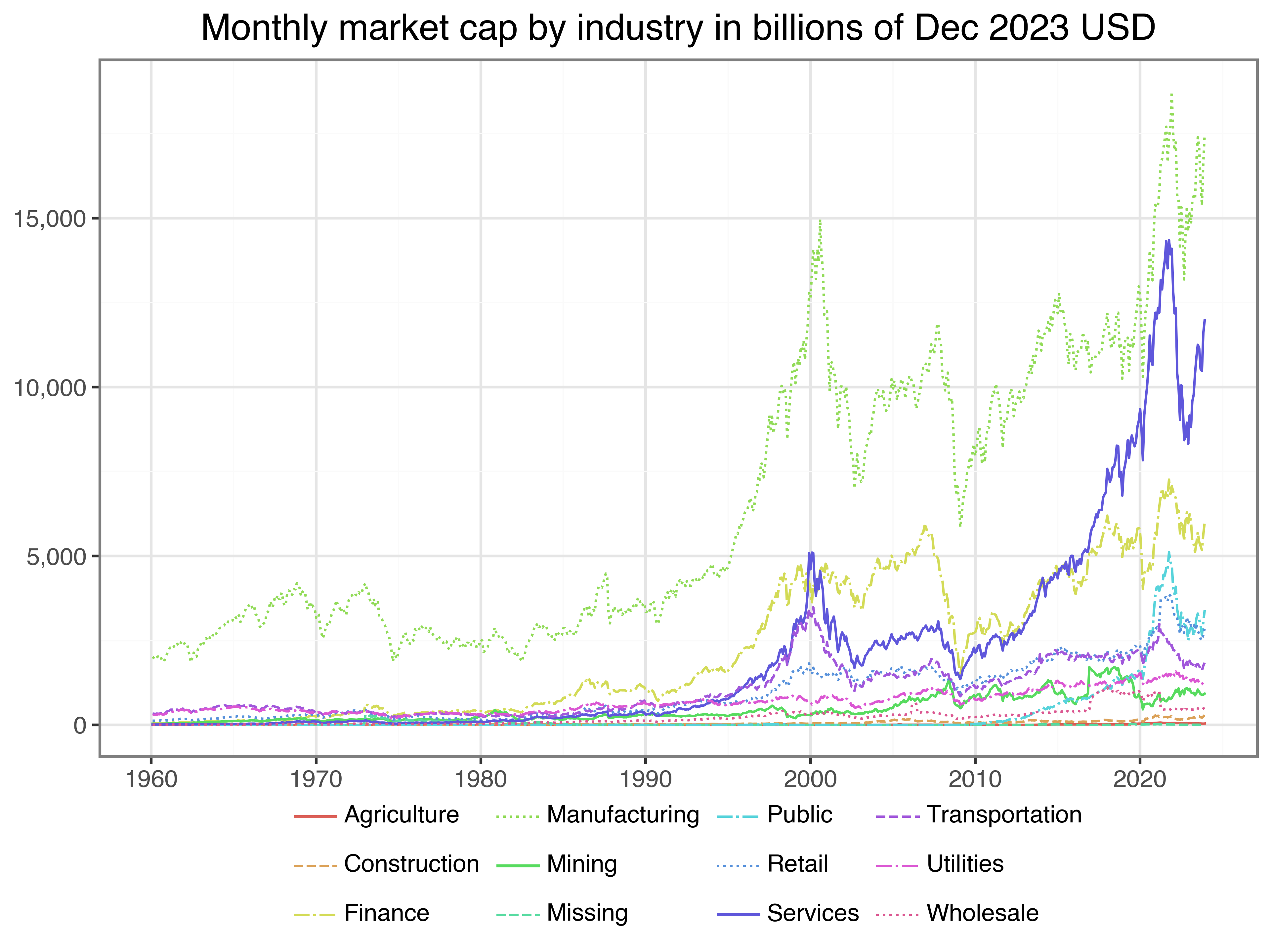

Figure 4: The figure shows the total Market capitalization in billion USD, adjusted for consumer price index changes such that the values on the y-axis reflect the buying power of billion USD in December 2023.

Daily CRSP Data

Before we turn to accounting data, we provide a proposal for downloading daily CRSP data with the same filters used for the monthly data (i.e., using information from stksecurityinfohist). While the monthly data from above typically fit into your memory and can be downloaded in a meaningful amount of time, this is usually not true for daily return data. The daily CRSP data file is substantially larger than monthly data and can exceed 20 GB. This has two important implications: you cannot hold all the daily return data in your memory (hence it is not possible to copy the entire dataset to your local database), and in our experience, the download usually crashes (or never stops) because it is too much data for the WRDS cloud to prepare and send to your Python session.

There is a solution to this challenge. As with many big data problems, you can split up the big task into several smaller tasks that are easier to handle. That is, instead of downloading data about all stocks at once, download the data in small batches of stocks consecutively. Such operations can be implemented in for-loops, where we download, prepare, and store the data for a small number of stocks in each iteration. This operation might nonetheless take around 5 minutes, depending on your internet connection. To keep track of the progress, we create ad-hoc progress updates using print(). Notice that we also use the method to_sql() here with the option to append the new data to an existing table, when we process the second and all following batches. As for the monthly CRSP data, there is no need to adjust for delisting returns in the daily CRSP data since July 2022.

factors_ff3_daily = pd.read_sql(
  sql="SELECT * FROM factors_ff3_daily", 
  con=tidy_finance,
  parse_dates={"date"}
)

permnos = pd.read_sql(
  sql="SELECT DISTINCT permno FROM crsp.stksecurityinfohist", 
  con=wrds,
  dtype={"permno": int}
)

permnos = list(permnos["permno"].astype(str))
  
batch_size = 500
batches = np.ceil(len(permnos)/batch_size).astype(int)
  
for j in range(1, batches+1):  
    
  permno_batch = permnos[
    ((j-1)*batch_size):(min(j*batch_size, len(permnos)))
  ]
  
  permno_batch_formatted = (
    ", ".join(f"'{permno}'" for permno in permno_batch)
  )
  permno_string = f"({permno_batch_formatted})"
  
  crsp_daily_sub_query = (
    "SELECT dsf.permno, dlycaldt AS date, dlyret AS ret "
      "FROM crsp.dsf_v2 AS dsf "
      "INNER JOIN crsp.stksecurityinfohist AS ssih "
      "ON dsf.permno = ssih.permno AND "
         "ssih.secinfostartdt <= dsf.dlycaldt AND "
         "dsf.dlycaldt <= ssih.secinfoenddt "
      f"WHERE dsf.permno IN {permno_string} "
           f"AND dlycaldt BETWEEN '{start_date}' AND '{end_date}' "
            "AND ssih.sharetype = 'NS' "
            "AND ssih.securitytype = 'EQTY' "  
            "AND ssih.securitysubtype = 'COM' " 
            "AND ssih.usincflg = 'Y' " 
            "AND ssih.issuertype in ('ACOR', 'CORP') " 
            "AND ssih.primaryexch in ('N', 'A', 'Q') "
            "AND ssih.conditionaltype in ('RW', 'NW') "
            "AND ssih.tradingstatusflg = 'A'"
  )
    
  crsp_daily_sub = (pd.read_sql_query(
      sql=crsp_daily_sub_query,
      con=wrds,
      dtype={"permno": int},
      parse_dates={"date"}
    )
    .dropna()
   )

  if not crsp_daily_sub.empty:
    
      crsp_daily_sub = (crsp_daily_sub
        .merge(factors_ff3_daily[["date", "rf"]], 
               on="date", how="left")
        .assign(
          ret_excess = lambda x: 
            ((x["ret"] - x["rf"]).clip(lower=-1))
        )
        .get(["permno", "date", "ret_excess"])
      )
        
      if j == 1:
        if_exists_string = "replace"
      else:
        if_exists_string = "append"

      crsp_daily_sub.to_sql(
        name="crsp_daily", 
        con=tidy_finance, 
        if_exists=if_exists_string, 
        index=False
      )
            
  print(f"Batch {j} out of {batches} done ({(j/batches)*100:.2f}%)\n")

Eventually, we end up with more than 71 million rows of daily return data. Note that we only store the identifying information that we actually need, namely permno and date alongside the excess returns. We thus ensure that our local database contains only the data that we actually use.

To download the daily CRSP data via the tidyfinance package, you can call:

crsp_daily = tf.download_data(
  domain="wrds",
  dataset="crsp_daily",
  start_date = start_date,
  end_date = end_date
)

Note that you need at least 16 GB of memory to hold all the daily CRSP returns in memory. We hence recommend to use loop the function over different date periods and store the results.

Preparing Compustat Data

Firm accounting data are an important source of information that we use in portfolio analyses in subsequent chapters. The commonly used source for firm financial information is Compustat provided by S&P Global Market Intelligence, which is a global data vendor that provides financial, statistical, and market information on active and inactive companies throughout the world. For US and Canadian companies, annual history is available back to 1950 and quarterly as well as monthly histories date back to 1962.

To access Compustat data, we can again tap WRDS, which hosts the funda table that contains annual firm-level information on North American companies. We follow the typical filter conventions and pull only data that we actually need: (i) we get only records in industrial data format, which includes companies that are primarily involved in manufacturing, services, and other non-financial business activities,³, (ii) in the standard format (i.e., consolidated information in standard presentation), (iii) reported in USD,⁴ and (iv) only data in the desired time window.

compustat_query = (
  "SELECT gvkey, datadate, seq, ceq, at, lt, txditc, txdb, itcb,  pstkrv, "
         "pstkl, pstk, capx, oancf, sale, cogs, xint, xsga "
    "FROM comp.funda "
    "WHERE indfmt = 'INDL' "
          "AND datafmt = 'STD' "
          "AND consol = 'C' "
          "AND curcd = 'USD' "
         f"AND datadate BETWEEN '{start_date}' AND '{end_date}'"
)

compustat = pd.read_sql_query(
  sql=compustat_query,
  con=wrds,
  dtype={"gvkey": str},
  parse_dates={"datadate"}
)

Next, we calculate the book value of preferred stock and equity be and the operating profitability op inspired by the variable definitions in Kenneth French’s data library. Note that we set negative or zero equity to missing, which is a common practice when working with book-to-market ratios (see Fama and French 1992 for details).

compustat = (compustat
  .assign(
    be=lambda x: 
      (x["seq"].combine_first(x["ceq"]+x["pstk"])
       .combine_first(x["at"]-x["lt"])+
       x["txditc"].combine_first(x["txdb"]+x["itcb"]).fillna(0)-
       x["pstkrv"].combine_first(x["pstkl"])
       .combine_first(x["pstk"]).fillna(0))
  )
  .assign(
    be=lambda x: x["be"].apply(lambda y: np.nan if y <= 0 else y)
  )
  .assign(
    op=lambda x: 
      ((x["sale"]-x["cogs"].fillna(0)- 
        x["xsga"].fillna(0)-x["xint"].fillna(0))/x["be"])
  )
)

We keep only the last available information for each firm-year group (by using the tail(1) pandas function for each group). Note that datadate defines the time the corresponding financial data refers to (e.g., annual report as of December 31, 2022). Therefore, datadate is not the date when data was made available to the public. Check out the Exercises for more insights into the peculiarities of datadate.

compustat = (compustat
  .assign(year=lambda x: pd.DatetimeIndex(x["datadate"]).year)
  .sort_values("datadate")
  .groupby(["gvkey", "year"])
  .tail(1)
  .reset_index()
)

We also compute the investment ratio (inv) according to Kenneth French’s variable definitions as the change in total assets from one fiscal year to another. Note that we again use the approach using joins as introduced with the CRSP data above to construct lagged assets.

compustat_lag = (compustat
  .get(["gvkey", "year", "at"])
  .assign(year=lambda x: x["year"]+1)
  .rename(columns={"at": "at_lag"})
)

compustat = (compustat
  .merge(compustat_lag, how="left", on=["gvkey", "year"])
  .assign(inv=lambda x: x["at"]/x["at_lag"]-1)
  .assign(inv=lambda x: np.where(x["at_lag"] <= 0, np.nan, x["inv"]))
)

With the last step, we are already done preparing the firm fundamentals. Thus, we can store them in our local database.

(compustat
  .to_sql(name="compustat", 
          con=tidy_finance, 
          if_exists="replace",
          index=False)
)

The tidyfinance package provides a shortcut for these processing steps as well:

compustat = tf.download_data(
  domain="wrds",
  dataset="compustat_annual",
  start_date = start_date,
  end_date = end_date
)

Merging CRSP with Compustat

Unfortunately, CRSP and Compustat use different keys to identify stocks and firms. CRSP uses permno for stocks, while Compustat uses gvkey to identify firms. Fortunately, a curated matching table on WRDS allows us to merge CRSP and Compustat, so we create a connection to the CRSP-Compustat Merged table (provided by CRSP). The linking table contains links between CRSP and Compustat identifiers from various approaches. However, we need to make sure that we keep only relevant and correct links, again following the description outlined in Bali, Engle, and Murray (2016). Note also that currently active links have no end date, so we just enter the current date via the SQL verb CURRENT_DATE.

ccm_linking_table_query = (
  "SELECT lpermno AS permno, gvkey, linkdt, "
         "COALESCE(linkenddt, CURRENT_DATE) AS linkenddt "
    "FROM crsp.ccmxpf_linktable "
    "WHERE linktype IN ('LU', 'LC') "
          "AND linkprim IN ('P', 'C')"
)

ccm_linking_table = pd.read_sql_query(
  sql=ccm_linking_table_query,
  con=wrds,
  dtype={"permno": int, "gvkey": str},
  parse_dates={"linkdt", "linkenddt"}
)

To fetch these links via tidyfinance, you can call:

ccm_links = tf.download_data(domain="wrds", dataset="ccm_links")

We use these links to create a new table with a mapping between stock identifier, firm identifier, and month. We then add these links to the Compustat gvkey to our monthly stock data.

ccm_links = (crsp_monthly
  .merge(ccm_linking_table, how="inner", on="permno")
  .query("~gvkey.isnull() & (date >= linkdt) & (date <= linkenddt)")
  .get(["permno", "gvkey", "date"])
)

crsp_monthly = (crsp_monthly
  .merge(ccm_links, how="left", on=["permno", "date"])
)

As the last step, we update the previously prepared monthly CRSP file with the linking information in our local database.

(crsp_monthly
  .to_sql(name="crsp_monthly", 
          con=tidy_finance, 
          if_exists="replace",
          index=False)
)

Before we close this chapter, let us look at an interesting descriptive statistic of our data. As the book value of equity plays a crucial role in many asset pricing applications, it is interesting to know for how many of our stocks this information is available. Hence, Figure 5 plots the share of securities with book equity values for each exchange. It turns out that the coverage is pretty bad for AMEX- and NYSE-listed stocks in the 1960s but hovers around 80 percent for all periods thereafter. We can ignore the erratic coverage of securities that belong to the other category since there is only a handful of them anyway in our sample.

share_with_be = (crsp_monthly
  .assign(year=lambda x: pd.DatetimeIndex(x["date"]).year)
  .sort_values("date")
  .groupby(["permno", "year"])
  .tail(1)
  .reset_index()
  .merge(compustat, how="left", on=["gvkey", "year"])
  .groupby(["exchange", "year"])
  .apply(
    lambda x: pd.Series({
    "share": x["permno"][~x["be"].isnull()].nunique()/x["permno"].nunique()
    })
  )
  .reset_index()
)

share_with_be_figure = (
  ggplot(
    share_with_be, 
    aes(x="year", y="share", color="exchange", linetype="exchange")
  )
  + geom_line()
  + labs(
      x="", y="", color="", linetype="",
      title="Share of securities with book equity values by exchange"
    )
  + scale_y_continuous(labels=percent_format())
  + coord_cartesian(ylim=(0, 1))
)
share_with_be_figure.show()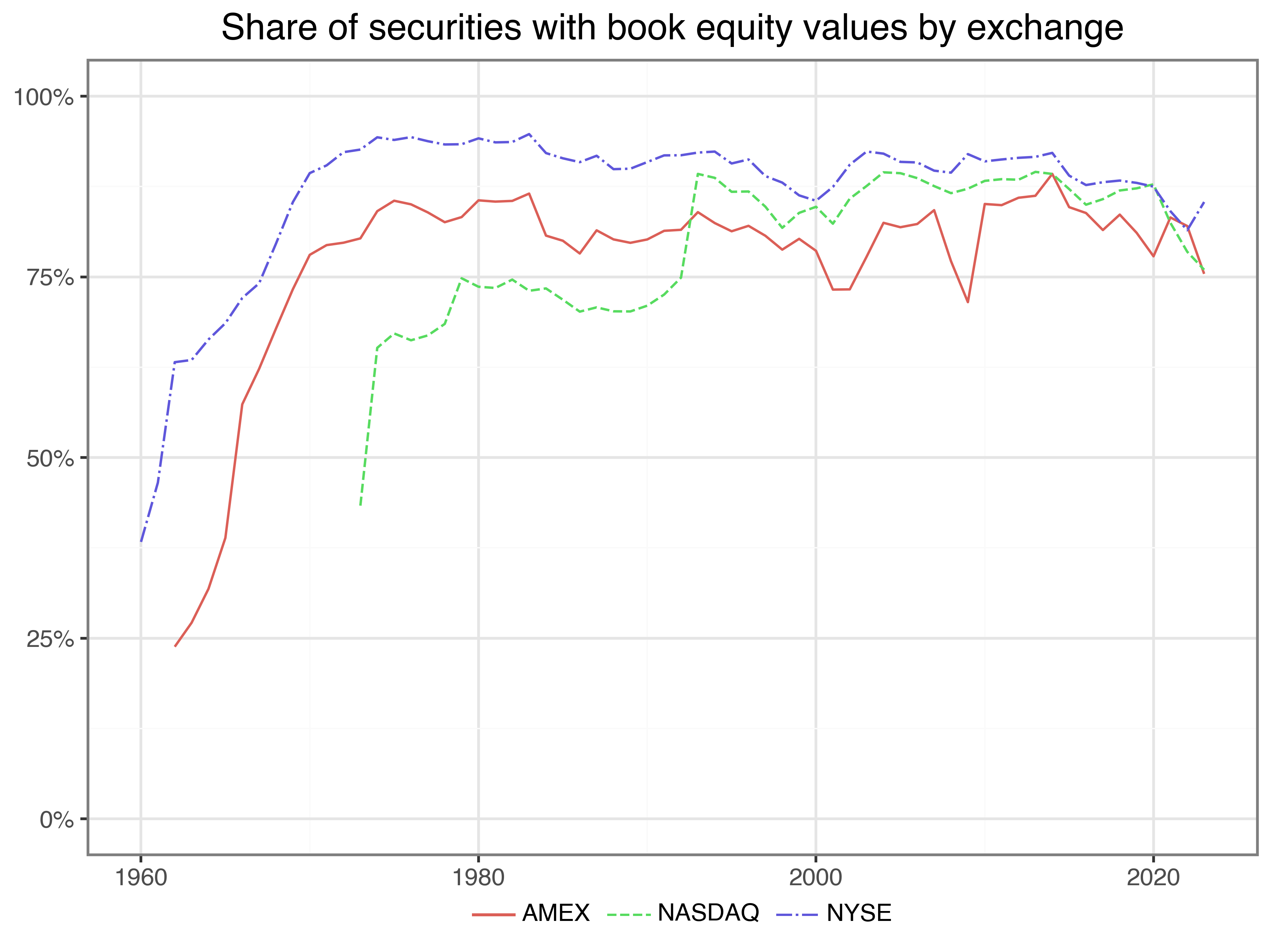

Figure 5: The figure shows the end-of-year share of securities with book equity values by listing exchange.

Key Takeaways

• WRDS provides secure access to essential financial databases like CRSP and Compustat, which are critical for empirical finance research.
• CRSP data provides return, market capitalization and industry data for US common stocks listed on NYSE, NASDAQ, or AMEX.
• Compustat provides firm-level accounting data such as book equity, profitability, and investment.
• The tidyfinance Python package streamlines all major data download and processing steps, making it easy to replicate and scale financial data analysis.

Exercises

1. Compute mkt_cap_lag using shift() rather than using joins as above. Filter out all the rows where the lag-based market capitalization measure is different from the one we computed above. Why are the two measures different?
2. Plot the average market capitalization of firms for each exchange and industry, respectively, over time. What do you find?
3. In the compustat table, datadate refers to the date to which the fiscal year of a corresponding firm refers. Count the number of observations in Compustat by month of this date variable. What do you find? What does the finding suggest about pooling observations with the same fiscal year?
4. Go back to the original Compustat and extract rows where the same firm has multiple rows for the same fiscal year. What is the reason for these observations?
5. Keep the last observation of crsp_monthly by year and join it with the compustat table. Create the following plots: (i) aggregate book equity by exchange over time and (ii) aggregate annual book equity by industry over time. Do you notice any different patterns to the corresponding plots based on market capitalization?
6. Repeat the analysis of market capitalization for book equity, which we computed from the Compustat data. Then, use the matched sample to plot book equity against market capitalization. How are these two variables related?

References

Bali, Turan G, Robert F Engle, and Scott Murray. 2016. Empirical asset pricing: The cross section of stock returns. John Wiley & Sons. https://doi.org/10.1002/9781118445112.stat07954.

Bayer, Michael. 2012. “SQLAlchemy.” In The Architecture of Open Source Applications Volume II: Structure, Scale, and a Few More Fearless Hacks, edited by Amy Brown and Greg Wilson. aosabook.org. http://aosabook.org/en/sqlalchemy.html.

Fama, Eugene F., and Kenneth R. French. 1992. “The cross-section of expected stock returns.” The Journal of Finance 47 (2): 427–65. https://doi.org/2329112.

———. 1997. “Industry Costs of Equity.” Journal of Financial Economics 43 (2): 153–93. https://doi.org/10.1016/s0304-405x(96)00896-3.

Footnotes

1. An alternative to establish a connection to WRDS is to use the WRDS-Py library. We chose to work with sqlalchemy (Bayer 2012) to show how to access PostgreSQL engines in general.

2. These three criteria jointly replicate the filter exchcd %in% c(1, 2, 3, 31, 32, 33) used for the legacy version of CRSP. If you do not want to include stocks at issuance, you can set the conditionaltype == "RW", which is equivalent to the restriction of exchcd %in% c(1, 2, 3) with the old CRSP format.

3. Companies that operate in the banking, insurance, or utilities sector typically report in different industry formats that reflect their specific regulatory requirements.

4. Compustat also contains reports in CAD, which can lead a currency mismatch, e.g., when relating book equity to market equity.