import pandas as pd
import numpy as np
import tidyfinance as tf
import sqlite3
import httpimport

from plotnine import *
from sqlalchemy import create_engine
from mizani.breaks import date_breaks
from mizani.formatters import date_format, comma_formatTRACE and FISD
Note
You are reading Tidy Finance with Python. You can find the equivalent chapter for the sibling Tidy Finance with R here.
In this chapter, we dive into the US corporate bond market. Bond markets are far more diverse than stock markets, as most issuers have multiple bonds outstanding simultaneously with potentially very different indentures. This market segment is exciting due to its size (roughly ten trillion USD outstanding), heterogeneity of issuers (as opposed to government bonds), market structure (mostly over-the-counter trades), and data availability. We introduce how to use bond characteristics from FISD and trade reports from TRACE and provide code to download and clean TRACE in Python.
Many researchers study liquidity in the US corporate bond market, with notable contributions from Bessembinder, Maxwell, and Venkataraman (2006), Edwards, Harris, and Piwowar (2007), and O’Hara and Zhou (2021), among many others. We do not cover bond returns here, but you can compute them from TRACE data. Instead, we refer to studies on the topic such as Bessembinder et al. (2008), Bai, Bali, and Wen (2019), and Kelly, Palhares, and Pruitt (2021) and a survey by Huang and Shi (2021).
This chapter also draws on the resources provided by the project Open Source Bond Asset Pricing and their related publication, i.e., Dickerson, Mueller, and Robotti (2023). We encourage you to visit their website to check out the additional resources they provide. Moreover, WRDS provides bond returns computed from TRACE data at a monthly frequency.
The current chapter relies on the following set of Python packages.
Compared to previous chapters, we load httpimport (Torakis 2023) to source code provided in the public Gist. Note that you should be careful with loading anything from the web via this method, and it is highly discouraged to use any unsecured “HTTP” links. Also, you might encounter a problem when using this from a corporate computer that prevents downloading data through a firewall.
Bond Data from WRDS
Both bond databases we need are available on WRDS to which we establish the PostgreSQL connection described in WRDS, CRSP, and Compustat. Additionally, we connect to our local SQLite-database to store the data we download.
import os
from dotenv import load_dotenv
load_dotenv()

connection_string = (
  "postgresql+psycopg2://"
  f"{os.getenv('WRDS_USER')}:{os.getenv('WRDS_PASSWORD')}"
  "@wrds-pgdata.wharton.upenn.edu:9737/wrds"
)

wrds = create_engine(connection_string, pool_pre_ping=True)

tidy_finance = sqlite3.connect(database="data/tidy_finance_python.sqlite")
Mergent FISD
For research on US corporate bonds, the Mergent Fixed Income Securities Database (FISD) is the primary resource for bond characteristics. There is a detailed manual on WRDS, so we only cover the necessary subjects here. FISD data comes in two main variants, namely, centered on issuers or issues. In either case, the most useful identifiers are CUSIPs. 9-digit CUSIPs identify securities issued by issuers. The issuers can be identified from the first six digits of a security CUSIP, which is also called a 6-digit CUSIP. Both stocks and bonds have CUSIPs. This connection would, in principle, allow matching them easily, but due to changing issuer details, this approach only yields small coverage.
We use the issue-centered version of FISD to identify the subset of US corporate bonds that meet the standard criteria (Bessembinder, Maxwell, and Venkataraman 2006). The WRDS table fisd_mergedissue contains most of the information we need on a 9-digit CUSIP level. Due to the diversity of corporate bonds, details in the indenture vary significantly. We focus on common bonds that make up the majority of trading volume in this market without diverging too much in indentures.
The following chunk connects to the data and selects the bond sample to remove certain bond types that are less commonly used (see, e.g., Dick-Nielsen, Feldhütter, and Lando 2012; O’Hara and Zhou 2021, among many others). In particular, we use the filters listed below. Note that we also treat missing values in these flags.
- Keep only senior bonds (
security_level = 'SEN'). - Exclude bonds which are secured lease obligations (
slob = 'N' OR slob IS NULL). - Exclude secured bonds (
security_pledge IS NULL). - Exclude asset-backed bonds (
asset_backed = 'N' OR asset_backed IS NULL). - Exclude defeased bonds (
(defeased = 'N' OR defeased IS NULL) AND defeased_date IS NULL). - Keep only the bond types US Corporate Debentures (
'CDEB'), US Corporate Medium Term Notes ('CMTN'), US Corporate Zero Coupon Notes and Bonds ('CMTZ','CZ'), and US Corporate Bank Note ('USBN'). - Exclude bonds that are payable in kind (
(pay_in_kind != 'Y' OR pay_in_kind IS NULL) AND pay_in_kind_exp_date IS NULL). - Exclude foreign (
yankee == "N" OR is.na(yankee)) and Canadian issuers (canadian = 'N' OR canadian IS NULL). - Exclude bonds denominated in foreign currency (
foreign_currency = 'N'). - Keep only fixed (
F) and zero (Z) coupon bonds with additional requirements offix_frequency IS NULL,coupon_change_indicator = 'N'and annual, semi-annual, quarterly, or monthly interest frequencies. - Exclude bonds that were issued under SEC Rule 144A (
rule_144a = 'N'). - Exlcude privately placed bonds (
private_placement = 'N' OR private_placement IS NULL). - Exclude defaulted bonds (
defaulted = 'N' AND filing_date IS NULL AND settlement IS NULL). - Exclude convertible (
convertible = 'N'), putable (putable = 'N' OR putable IS NULL), exchangeable (exchangeable = 'N' OR exchangeable IS NULL), perpetual (perpetual = 'N'), or preferred bonds (preferred_security = 'N' OR preferred_security IS NULL). - Exclude unit deal bonds (
(unit_deal = 'N' OR unit_deal IS NULL)).
fisd_query = (
  "SELECT complete_cusip, maturity, offering_amt, offering_date, "
         "dated_date, interest_frequency, coupon, last_interest_date, "
         "issue_id, issuer_id "
    "FROM fisd.fisd_mergedissue "
    "WHERE security_level = 'SEN' "
          "AND (slob = 'N' OR slob IS NULL) "
          "AND security_pledge IS NULL "
          "AND (asset_backed = 'N' OR asset_backed IS NULL) "
          "AND (defeased = 'N' OR defeased IS NULL) "
          "AND defeased_date IS NULL "
          "AND bond_type IN ('CDEB', 'CMTN', 'CMTZ', 'CZ', 'USBN') "
          "AND (pay_in_kind != 'Y' OR pay_in_kind IS NULL) "
          "AND pay_in_kind_exp_date IS NULL "
          "AND (yankee = 'N' OR yankee IS NULL) "
          "AND (canadian = 'N' OR canadian IS NULL) "
          "AND foreign_currency = 'N' "
          "AND coupon_type IN ('F', 'Z') "
          "AND fix_frequency IS NULL "
          "AND coupon_change_indicator = 'N' "
          "AND interest_frequency IN ('0', '1', '2', '4', '12') "
          "AND rule_144a = 'N' "
          "AND (private_placement = 'N' OR private_placement IS NULL) "
          "AND defaulted = 'N' "
          "AND filing_date IS NULL "
          "AND settlement IS NULL "
          "AND convertible = 'N' "
          "AND exchange IS NULL "
          "AND (putable = 'N' OR putable IS NULL) "
          "AND (unit_deal = 'N' OR unit_deal IS NULL) "
          "AND (exchangeable = 'N' OR exchangeable IS NULL) "
          "AND perpetual = 'N' "
          "AND (preferred_security = 'N' OR preferred_security IS NULL)"
)

fisd = pd.read_sql_query(
  sql=fisd_query,
  con=wrds,
  dtype={"complete_cusip": str, "interest_frequency": str,
         "issue_id": int, "issuer_id": int},
  parse_dates={"maturity", "offering_date",
               "dated_date", "last_interest_date"}
)
We also pull issuer information from fisd_mergedissuer regarding the industry and country of the firm that issued a particular bond. Then, we filter to include only US-domiciled firms’ bonds. We match the data by issuer_id.
fisd_issuer_query = (
  "SELECT issuer_id, sic_code, country_domicile "
    "FROM fisd.fisd_mergedissuer"
)

fisd_issuer = pd.read_sql_query(
  sql=fisd_issuer_query,
  con=wrds,
  dtype={"issuer_id": int, "sic_code": str, "country_domicile": str}
)

fisd = (fisd
  .merge(fisd_issuer, how="inner", on="issuer_id")
  .query("country_domicile == 'USA'")
  .drop(columns="country_domicile")
)
To download the FISD data with the above filters and processing steps, you can use the tidyfinance package. Note that you might have to set the login credentials for WRDS first using tf.set_wrds_credentials().
fisd = tf.download_data(domain="wrds", dataset="fisd")Finally, we save the bond characteristics to our local database. This selection of bonds also constitutes the sample for which we will collect trade reports from TRACE below.
(fisd
  .to_sql(name="fisd",
          con=tidy_finance,
          if_exists="replace",
          index=False)
)
The FISD database also contains other data. The issue-based file contains information on covenants, i.e., restrictions included in bond indentures to limit specific actions by firms (e.g., Handler, Jankowitsch, and Weiss 2021). The FISD redemption database also contains information on callable bonds. Moreover, FISD also provides information on bond ratings. We do not need either here.
TRACE
The Financial Industry Regulatory Authority (FINRA) provides the Trade Reporting and Compliance Engine (TRACE). In TRACE, dealers that trade corporate bonds must report such trades individually. Hence, we observe trade messages in TRACE that contain information on the bond traded, the trade time, price, and volume. TRACE comes in two variants: standard and enhanced TRACE. We show how to download and clean enhanced TRACE as it contains uncapped volume, a crucial quantity missing in the standard distribution. Moreover, enhanced TRACE also provides information on the respective parties’ roles and the direction of the trade report. These items become essential in cleaning the messages.
Why do we repeatedly talk about cleaning TRACE? Trade messages are submitted within a short time window after a trade is executed (less than 15 minutes). These messages can contain errors, and the reporters subsequently correct them or they cancel a trade altogether. The cleaning needs are described by Dick-Nielsen (2009) in detail, and Dick-Nielsen (2014) shows how to clean the enhanced TRACE data using SAS. We do not go into the cleaning steps here, since the code is lengthy and is not our focus here. However, downloading and cleaning enhanced TRACE data is straightforward with our setup.
We store code for cleaning enhanced TRACE with Python on the following GitHub Gist. Clean Enhanced TRACE with Python also contains the code for reference. We only need to source the code from the Gist, which we can do with the code below using httpimport. In the chunk, we explicitly load the necessary function interpreting the Gist as a module (i.e., you could also use it as a module and precede the function calls with the module’s name). Alternatively, you can also go to the Gist, download it, and manually execute it. The clean_enhanced_trace() function takes a vector of CUSIPs, a connection to WRDS explained in WRDS, CRSP, and Compustat, and a start and end date, respectively.
gist_url = (
  "https://gist.githubusercontent.com/patrick-weiss/"
  "86ddef6de978fbdfb22609a7840b5d8b/raw/"
  "8fbcc6c6f40f537cd3cd37368be4487d73569c6b/"
)

with httpimport.remote_repo(gist_url):
  from clean_enhanced_TRACE_python import clean_enhanced_trace
The TRACE database is considerably large. Therefore, we only download subsets of data at once. Specifying too many CUSIPs over a long time horizon will result in very long download times and a potential failure due to the size of the request to WRDS. The size limit depends on many parameters, and we cannot give you a guideline here. For the applications in this book, we need data around the Paris Agreement in December 2015 and download the data in sets of 1000 bonds, which we define below.
cusips = list(fisd["complete_cusip"].unique())
batch_size = 1000
batches = np.ceil(len(cusips)/batch_size).astype(int)
Finally, we run a loop in the same style as in WRDS, CRSP, and Compustat where we download daily returns from CRSP. For each of the CUSIP sets defined above, we call the cleaning function and save the resulting output. We add new data to the existing table for batch two and all following batches.
for j in range(1, batches + 1):

  cusip_batch = cusips[
    ((j-1)*batch_size):(min(j*batch_size, len(cusips)))
  ]

  cusip_batch_formatted = ", ".join(f"'{cusip}'" for cusip in cusip_batch)
  cusip_string = f"({cusip_batch_formatted})"

  trace_enhanced_sub = clean_enhanced_trace(
    cusips=cusip_string,
    connection=wrds,
    start_date="'01/01/2014'",
    end_date="'11/30/2016'"
  )

  if not trace_enhanced_sub.empty:
      if j == 1:
        if_exists_string = "replace"
      else:
        if_exists_string = "append"

      trace_enhanced_sub.to_sql(
        name="trace_enhanced",
        con=tidy_finance,
        if_exists=if_exists_string,
        index=False
      )

  print(f"Batch {j} out of {batches} done ({(j/batches)*100:.2f}%)\n")
If you want to download the prepared enhanced TRACE data for selected bonds via the tidyfinance package, you can call, e.g.:
tf.download_data(
  domain="wrds",
  dataset="trace_enhanced",
  cusips=["00101JAH9"],
  start_date="2019-01-01",
  end_date="2021-12-31"
)
Insights into Corporate Bonds
While many news outlets readily provide information on stocks and the underlying firms, corporate bonds are not covered frequently. Additionally, the TRACE database contains trade-level information, potentially new to students. Therefore, we provide you with some insights by showing some summary statistics.
We start by looking into the number of bonds outstanding over time and compare it to the number of bonds traded in our sample. First, we compute the number of bonds outstanding for each quarter around the Paris Agreement from 2014 to 2016.
dates = pd.date_range(start="2014-01-01", end="2016-11-30", freq="Q")

bonds_outstanding = (pd.DataFrame({"date": dates})
  .merge(fisd[["complete_cusip"]], how="cross")
  .merge(fisd[["complete_cusip", "offering_date", "maturity"]],
         on="complete_cusip", how="left")
  .assign(offering_date=lambda x: x["offering_date"].dt.floor("D"),
          maturity=lambda x: x["maturity"].dt.floor("D"))
  .query("date >= offering_date & date <= maturity")
  .groupby("date")
  .size()
  .reset_index(name="count")
  .assign(type="Outstanding")
)
Next, we look at the bonds traded each quarter in the same period. Notice that we load the complete trace table from our database, as we only have a single part of it in the environment from the download loop above.
trace_enhanced = pd.read_sql_query(
  sql=("SELECT cusip_id, trd_exctn_dt, rptd_pr, entrd_vol_qt, yld_pt "
        "FROM trace_enhanced"),
  con=tidy_finance,
  parse_dates={"trd_exctn_dt"}
)

bonds_traded = (trace_enhanced
  .assign(
    date=lambda x: (
      (x["trd_exctn_dt"]-pd.offsets.MonthBegin(1))
        .dt.to_period("Q").dt.start_time
    )
  )
  .groupby("date")
  .aggregate(count=("cusip_id", "nunique"))
  .reset_index()
  .assign(type="Traded")
)
Finally, we plot the two time series in Figure 1.
bonds_combined = pd.concat(
  [bonds_outstanding, bonds_traded], ignore_index=True
)

bonds_figure = (
  ggplot(
    bonds_combined,
    aes(x="date", y="count", color="type", linetype="type")
  )
  + geom_line()
  + labs(
      x="", y="", color="", linetype="",
       title="Number of bonds outstanding and traded each quarter"
    )
  + scale_x_datetime(breaks=date_breaks("1 year"), labels=date_format("%Y"))
  + scale_y_continuous(labels=comma_format())
)
bonds_figure.draw()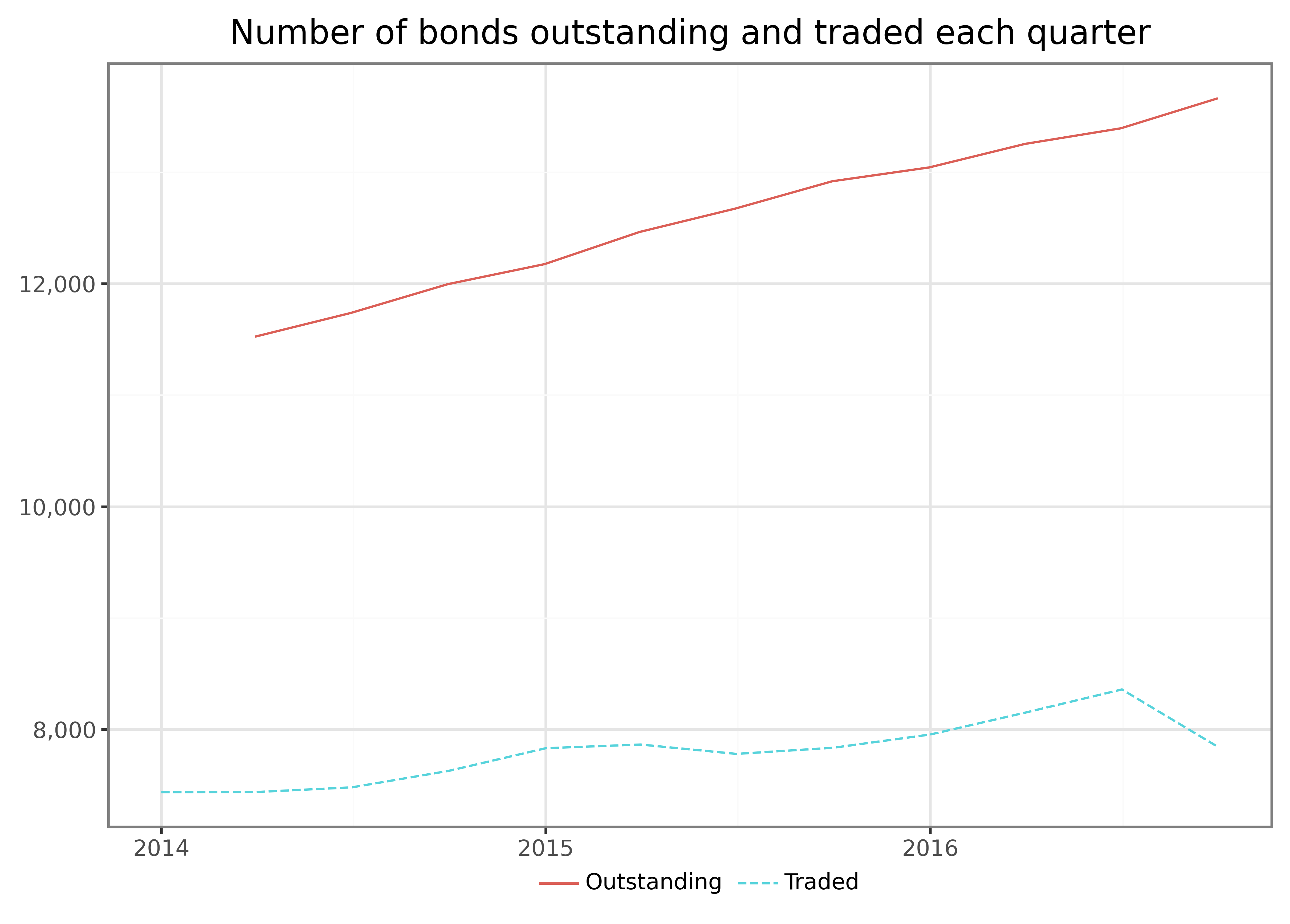
We see that the number of bonds outstanding increases steadily between 2014 and 2016. During our sample period of trade data, we see that the fraction of bonds trading each quarter is roughly 60 percent. The relatively small number of traded bonds means that many bonds do not trade through an entire quarter. This lack of trading activity illustrates the generally low level of liquidity in the corporate bond market, where it can be hard to trade specific bonds. Does this lack of liquidity mean that corporate bond markets are irrelevant in terms of their size? With over 7,500 traded bonds each quarter, it is hard to say that the market is small. However, let us also investigate the characteristics of issued corporate bonds. In particular, we consider maturity (in years), coupon, and offering amount (in million USD).
average_characteristics = (fisd
  .assign(
    maturity=lambda x: (x["maturity"] - x["offering_date"]).dt.days/365,
    offering_amt=lambda x: x["offering_amt"]/10**3
  )
  .melt(var_name="measure",
        value_vars=["maturity", "coupon", "offering_amt"],
        value_name="value")
  .dropna()
  .groupby("measure")["value"]
  .describe(percentiles=[.05, .50, .95])
  .drop(columns="count")
)
average_characteristics.round(2)| mean | std | min | 5% | 50% | 95% | max | |
|---|---|---|---|---|---|---|---|
| measure | |||||||
| coupon | 2.55 | 3.52 | 0.00 | 0.00 | 0.0 | 8.88 | 39.00 |
| maturity | 5.66 | 6.85 | -6.24 | 1.04 | 4.0 | 20.03 | 100.74 |
| offering_amt | 133.01 | 369.76 | 0.00 | 0.23 | 3.0 | 750.00 | 15000.00 |
We see that the average bond in our sample period has an offering amount of over 357 million USD with a median of 200 million USD, which both cannot be considered small. The average bond has a maturity of ten years and pays around 6 percent in coupons.
Finally, let us compute some summary statistics for the trades in this market. To this end, we show a summary based on aggregate information daily. In particular, we consider the trade size (in million USD) and the number of trades.
average_trade_size = (trace_enhanced
  .groupby("trd_exctn_dt")
  .aggregate(
    trade_size=("entrd_vol_qt", lambda x: (
      sum(x*trace_enhanced.loc[x.index, "rptd_pr"]/100)/10**6)
    ),
    trade_number=("trd_exctn_dt", "size")
  )
  .reset_index()
  .melt(id_vars=["trd_exctn_dt"], var_name="measure",
        value_vars=["trade_size", "trade_number"], value_name="value")
  .groupby("measure")["value"]
  .describe(percentiles=[.05, .50, .95])
  .drop(columns="count")
)
average_trade_size.round(0)| mean | std | min | 5% | 50% | 95% | max | |
|---|---|---|---|---|---|---|---|
| measure | |||||||
| trade_number | 25914.0 | 5444.0 | 439.0 | 17844.0 | 26051.0 | 34383.0 | 40839.0 |
| trade_size | 12968.0 | 3577.0 | 17.0 | 6128.0 | 13421.0 | 17850.0 | 21312.0 |
On average, nearly 26 billion USD of corporate bonds are traded daily in nearly 13,000 transactions. We can, hence, conclude that the corporate bond market is indeed significant in terms of trading volume and activity.
Key Takeaways
- The US corporate bond market is large, diverse, and primarily trades over-the-counter, making it an important yet complex subject of financial research.
- The Mergent FISD database on WRDS provides detailed bond characteristics, which are essential for selecting a representative sample of US corporate bonds.
- Enhanced TRACE data includes uncapped trade volumes and dealer roles, offering valuable insights into bond market liquidity and trade execution.
- Cleaning TRACE data is crucial, as trades may be corrected or canceled shortly after reporting, but automated functions in the
tidyfinancePython package simplify this task.
Exercises
- Compute the amount outstanding across all bonds over time. Make sure to subtract all matured bonds. How would you describe the resulting plot?
- Compute the number of days each bond is traded (accounting for the bonds’ maturities and issuances). Start by looking at the number of bonds traded each day in a graph similar to the one above. How many bonds trade on more than 75 percent of trading days?
- WRDS provides more information from Mergent FISD such as ratings in the table
fisd_ratings. Download the ratings table and plot the distribution of ratings for the different rating providers. How would you map the different providers to a common numeric rating scale?
References
Bai, Jennie, Turan G Bali, and Quan Wen. 2019. “Common risk factors in the cross-section of corporate bond returns.” Journal of Financial Economics 131 (3): 619–42. https://doi.org/10.1016/j.jfineco.2018.08.002.
Bessembinder, Hendrik, Kathleen M Kahle, William F Maxwell, and Danielle Xu. 2008. “Measuring abnormal bond performance.” Review of Financial Studies 22 (10): 4219–58. https://doi.org/10.1093/rfs/hhn105.
Bessembinder, Hendrik, William Maxwell, and Kumar Venkataraman. 2006. “Market transparency, liquidity externalities, and institutional trading costs in corporate bonds.” Journal of Financial Economics 82 (2): 251–88. https://doi.org/10.1016/j.jfineco.2005.10.002.
Dickerson, Alexander, Philippe Mueller, and Cesare Robotti. 2023. “Priced Risk in Corporate Bonds.” Journal of Financial Economics 150 (2): 103707. https://doi.org/10.1016/j.jfineco.2023.103707.
Dick-Nielsen, Jens. 2009. “Liquidity biases in TRACE.” The Journal of Fixed Income 19 (2): 43–55. https://doi.org/10.3905/jfi.2009.19.2.043.
———. 2014. “How to clean enhanced TRACE data.” Working Paper. https://ssrn.com/abstract=2337908.
Dick-Nielsen, Jens, Peter Feldhütter, and David Lando. 2012. “Corporate bond liquidity before and after the onset of the subprime crisis.” Journal of Financial Economics 103 (3): 471–92. https://doi.org/10.1016/j.jfineco.2014.06.001.
Edwards, Amy K., Lawrence E. Harris, and Michael S. Piwowar. 2007. “Corporate bond market transaction costs and transparency.” The Journal of Finance 62 (3): 1421–51. https://doi.org/10.1111/j.1540-6261.2007.01240.x.
Handler, Lukas, Rainer Jankowitsch, and Patrick Weiss. 2021. “Covenant prices of US corporate bonds.” Working Paper. https://dx.doi.org/10.2139/ssrn.3827385.
Huang, Jing-Zhi, and Zhan Shi. 2021. “What do we know about corporate bond returns?” Annual Review of Financial Economics 13 (1): 363–99. https://doi.org/10.1146/annurev-financial-110118-123129.
Kelly, Bryan T., Diogo Palhares, and Seth Pruitt. 2021. “Modeling corporate bond returns.” Working Paper. https://dx.doi.org/10.2139/ssrn.3720789.
O’Hara, Maureen, and Xing Alex Zhou. 2021. “Anatomy of a liquidity crisis: Corporate bonds in the COVID-19 crisis.” Journal of Financial Economics 142 (1): 46–68. https://doi.org/10.1016/j.jfineco.2021.05.052.
Torakis, John. 2023. “Httpimport: Module for Remote in-Memory Python Package/Module Loading Through HTTP.” https://pypi.org/project/httpimport/.