import pandas as pd
import numpy as np
import sqlite3
import statsmodels.api as sm

from plotnine import *
from mizani.formatters import percent_format
from regtabletotext import prettify_resultUnivariate Portfolio Sorts
Note
You are reading Tidy Finance with Python. You can find the equivalent chapter for the sibling Tidy Finance with R here.
In this chapter, we dive into portfolio sorts, one of the most widely used statistical methodologies in empirical asset pricing (e.g., Bali, Engle, and Murray 2016). The key application of portfolio sorts is to examine whether one or more variables can predict future excess returns. In general, the idea is to sort individual stocks into portfolios, where the stocks within each portfolio are similar with respect to a sorting variable, such as firm size. The different portfolios then represent well-diversified investments that differ in the level of the sorting variable. You can then attribute the differences in the return distribution to the impact of the sorting variable. We start by introducing univariate portfolio sorts (which sort based on only one characteristic) and tackle bivariate sorting in Value and Bivariate Sorts.
A univariate portfolio sort considers only one sorting variable \(x_{i,t-1}\). Here, \(i\) denotes the stock and \(t-1\) indicates that the characteristic is observable by investors at time \(t\). The objective is to assess the cross-sectional relation between \(x_{i,t-1}\) and, typically, stock excess returns \(r_{i,t}\) at time \(t\) as the outcome variable. To illustrate how portfolio sorts work, we use estimates for market betas from the previous chapter as our sorting variable.
The current chapter relies on the following set of Python packages.
Data Preparation
We start with loading the required data from our SQLite database introduced in Accessing and Managing Financial Data and WRDS, CRSP, and Compustat. In particular, we use the monthly CRSP sample as our asset universe. Once we form our portfolios, we use the Fama-French market factor returns to compute the risk-adjusted performance (i.e., alpha). beta is the dataframe with market betas computed in the previous chapter.
tidy_finance = sqlite3.connect(database="data/tidy_finance_python.sqlite")

crsp_monthly = (pd.read_sql_query(
    sql="SELECT permno, date, ret_excess, mktcap_lag FROM crsp_monthly",
    con=tidy_finance,
    parse_dates={"date"})
)

factors_ff3_monthly = pd.read_sql_query(
  sql="SELECT date, mkt_excess FROM factors_ff3_monthly",
  con=tidy_finance,
  parse_dates={"date"}
)

beta = (pd.read_sql_query(
    sql="SELECT permno, date, beta_monthly FROM beta",
    con=tidy_finance,
    parse_dates={"date"})
)
Sorting by Market Beta
Next, we merge our sorting variable with the return data. We use the one-month lagged betas as a sorting variable to ensure that the sorts rely only on information available when we create the portfolios. To lag stock beta by one month, we add one month to the current date and join the resulting information with our return data. This procedure ensures that month \(t\) information is available in month \(t+1\). You may be tempted to simply use a call such as crsp_monthly['beta_lag'] = crsp_monthly.groupby('permno')['beta'].shift(1) instead. This procedure, however, does not work correctly if there are implicit missing values in the time series.
beta_lag = (beta
  .assign(date=lambda x: x["date"]+pd.DateOffset(months=1))
  .get(["permno", "date", "beta_monthly"])
  .rename(columns={"beta_monthly": "beta_lag"})
  .dropna()
)

data_for_sorts = (crsp_monthly
  .merge(beta_lag, how="inner", on=["permno", "date"])
)
The first step to conduct portfolio sorts is to calculate periodic breakpoints that you can use to group the stocks into portfolios. For simplicity, we start with the median lagged market beta as the single breakpoint. We then compute the value-weighted returns for each of the two resulting portfolios, which means that the lagged market capitalization determines the weight in np.average().
beta_portfolios = (data_for_sorts
  .groupby("date")
  .apply(lambda x: (x.assign(
      portfolio=pd.qcut(
        x["beta_lag"], q=[0, 0.5, 1], labels=["low", "high"]))
    )
  )
  .reset_index(drop=True)
  .groupby(["portfolio","date"])
  .apply(lambda x: np.average(x["ret_excess"], weights=x["mktcap_lag"]))
  .reset_index(name="ret")
)
Performance Evaluation
We can construct a long-short strategy based on the two portfolios: buy the high-beta portfolio and, at the same time, short the low-beta portfolio. Thereby, the overall position in the market is net-zero, i.e., you do not need to invest money to realize this strategy in the absence of frictions.
beta_longshort = (beta_portfolios
  .pivot_table(index="date", columns="portfolio", values="ret")
  .reset_index()
  .assign(long_short=lambda x: x["high"]-x["low"])
)
We compute the average return and the corresponding standard error to test whether the long-short portfolio yields on average positive or negative excess returns. In the asset pricing literature, one typically adjusts for autocorrelation by using Newey and West (1987) \(t\)-statistics to test the null hypothesis that average portfolio excess returns are equal to zero. One necessary input for Newey-West standard errors is a chosen bandwidth based on the number of lags employed for the estimation. Researchers often default to choosing a pre-specified lag length of six months (which is not a data-driven approach). We do so in the fit() function by indicating the cov_type as HAC and providing the maximum lag length through an additional keywords dictionary.
model_fit = (sm.OLS.from_formula(
    formula="long_short ~ 1",
    data=beta_longshort
  )
  .fit(cov_type="HAC", cov_kwds={"maxlags": 6})
)
prettify_result(model_fit)
OLS Model:
long_short ~ 1
Coefficients:
Estimate Std. Error t-Statistic p-Value
Intercept 0.0 0.001 0.275 0.783
Summary statistics:
- Number of observations: 707
- R-squared: -0.000, Adjusted R-squared: -0.000
- F-statistic not available
The results indicate that we cannot reject the null hypothesis of average returns being equal to zero. Our portfolio strategy using the median as a breakpoint does not yield any abnormal returns. Is this finding surprising if you reconsider the CAPM? It certainly is. The CAPM yields that the high-beta stocks should yield higher expected returns. Our portfolio sort implicitly mimics an investment strategy that finances high-beta stocks by shorting low-beta stocks. Therefore, one should expect that the average excess returns yield a return that is above the risk-free rate.
Functional Programming for Portfolio Sorts
Now, we take portfolio sorts to the next level. We want to be able to sort stocks into an arbitrary number of portfolios. For this case, functional programming is very handy: we define a function that gives us flexibility concerning which variable to use for the sorting, denoted by sorting_variable. We use np.quantile() to compute breakpoints for n_portfolios. Then, we assign portfolios to stocks using the pd.cut() function. The output of the following function is a new column that contains the number of the portfolio to which a stock belongs.
In some applications, the variable used for the sorting might be clustered (e.g., at a lower bound of 0). Then, multiple breakpoints may be identical, leading to empty portfolios. Similarly, some portfolios might have a very small number of stocks at the beginning of the sample. Cases where the number of portfolio constituents differs substantially due to the distribution of the characteristics require careful consideration and, depending on the application, might require customized sorting approaches.
def assign_portfolio(data, sorting_variable, n_portfolios):
    """Assign portfolios to a bin between breakpoints."""

    breakpoints = np.quantile(
      data[sorting_variable].dropna(),
      np.linspace(0, 1, n_portfolios + 1),
      method="linear"
    )

    assigned_portfolios = pd.cut(
      data[sorting_variable],
      bins=breakpoints,
      labels=range(1, breakpoints.size),
      include_lowest=True,
      right=False
    )

    return assigned_portfolios
We can use the above function to sort stocks into ten portfolios each month using lagged betas and compute value-weighted returns for each portfolio. Note that we transform the portfolio column to a factor variable because it provides more convenience for the figure construction below.
beta_portfolios = (data_for_sorts
  .groupby("date")
  .apply(lambda x: x.assign(
      portfolio=assign_portfolio(x, "beta_lag", 10)
    )
  )
  .reset_index(drop=True)
  .groupby(["portfolio", "date"])
  .apply(lambda x: x.assign(
      ret=np.average(x["ret_excess"], weights=x["mktcap_lag"])
    )
  )
  .reset_index(drop=True)
  .merge(factors_ff3_monthly, how="left", on="date")
)
More Performance Evaluation
In the next step, we compute summary statistics for each beta portfolio. Namely, we compute CAPM-adjusted alphas, the beta of each beta portfolio, and average returns.
beta_portfolios_summary = (beta_portfolios
  .groupby("portfolio")
  .apply(lambda x: x.assign(
      alpha=sm.OLS.from_formula(
          formula="ret ~ 1 + mkt_excess",
          data=x
        ).fit().params[0],
      beta=sm.OLS.from_formula(
          formula="ret ~ 1 + mkt_excess",
          data=x
        ).fit().params[1],
      ret=x["ret"].mean()
    ).tail(1)
  )
  .reset_index(drop=True)
  .get(["portfolio", "alpha", "beta", "ret"])
)
Figure 1 illustrates the CAPM alphas of beta-sorted portfolios. It shows that low-beta portfolios tend to exhibit positive alphas, while high-beta portfolios exhibit negative alphas.
beta_portfolios_figure = (
  ggplot(
    beta_portfolios_summary,
    aes(x="portfolio", y="alpha", fill="portfolio")
  )
  + geom_bar(stat="identity")
  + labs(
      x="Portfolio", y="CAPM alpha", fill="Portfolio",
      title="CAPM alphas of beta-sorted portfolios"
    )
  + scale_y_continuous(labels=percent_format())
  + theme(legend_position="none")
)
beta_portfolios_figure.show()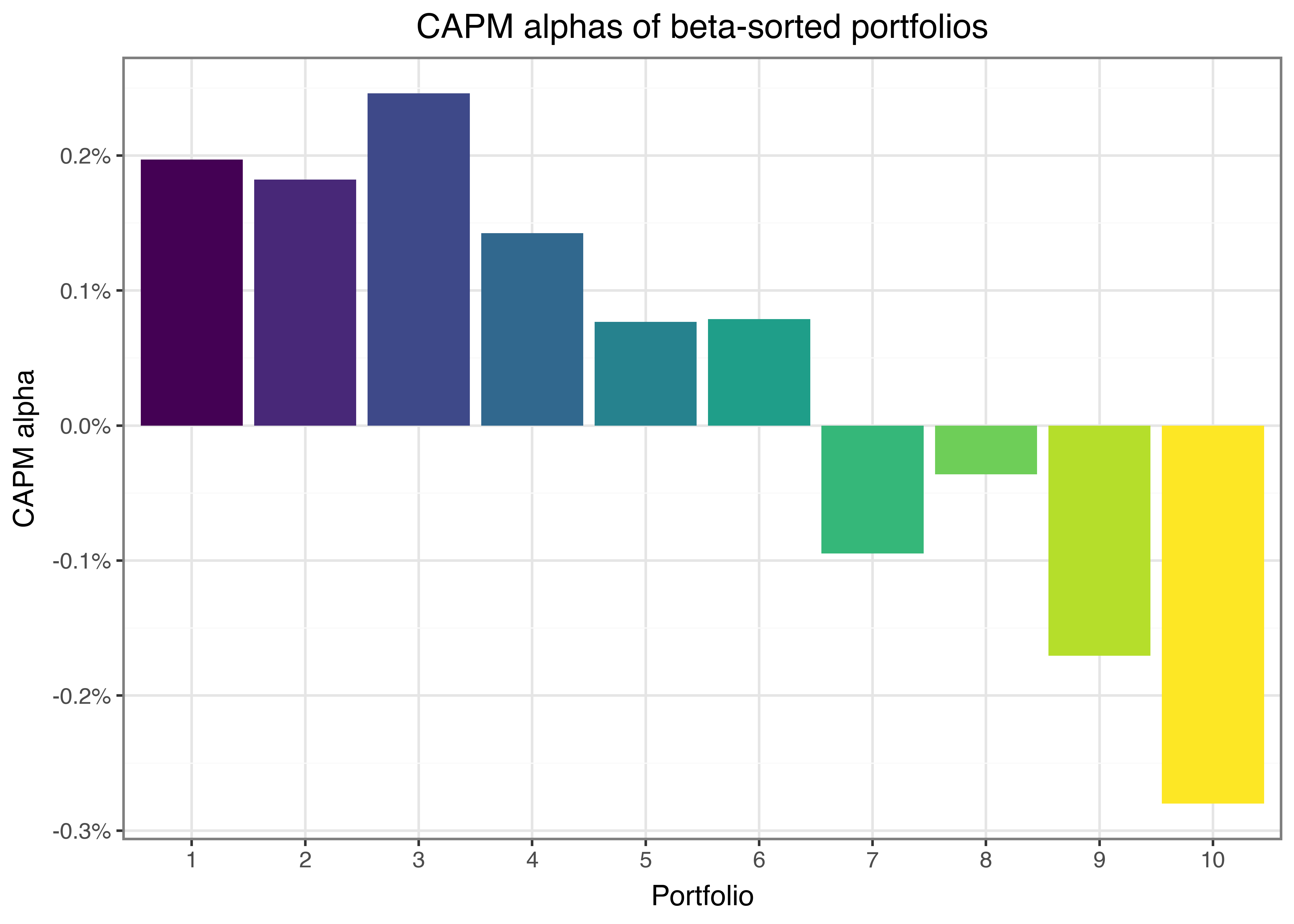
These results suggest a negative relation between beta and future stock returns, which contradicts the predictions of the CAPM. According to the CAPM, returns should increase with beta across the portfolios and risk-adjusted returns should be statistically indistinguishable from zero.
Security Market Line and Beta Portfolios
The CAPM predicts that our portfolios should lie on the security market line (SML). The slope of the SML is equal to the market risk premium and reflects the risk-return trade-off at any given time. Figure 2 illustrates the security market line: We see that (not surprisingly) the high-beta portfolio returns have a high correlation with the market returns. However, it seems like the average excess returns for high-beta stocks are lower than what the security market line implies would be an “appropriate” compensation for the high market risk.
sml_capm = (sm.OLS.from_formula(
    formula="ret ~ 1 + beta",
    data=beta_portfolios_summary
  )
  .fit()
  .params
)

sml_figure = (
  ggplot(
    beta_portfolios_summary,
    aes(x="beta", y="ret", color="portfolio")
  )
  + geom_point()
  + geom_abline(
      intercept=0, slope=factors_ff3_monthly["mkt_excess"].mean(), linetype="solid"
    )
  + geom_abline(
      intercept=sml_capm["Intercept"], slope=sml_capm["beta"], linetype="dashed"
    )
  + labs(
      x="Beta", y="Excess return", color="Portfolio",
      title="Average portfolio excess returns and beta estimates"
    )
  + scale_x_continuous(limits=(0, 2))
  + scale_y_continuous(
      labels=percent_format(),
      limits=(0, factors_ff3_monthly["mkt_excess"].mean()*2)
    )
)
sml_figure.show()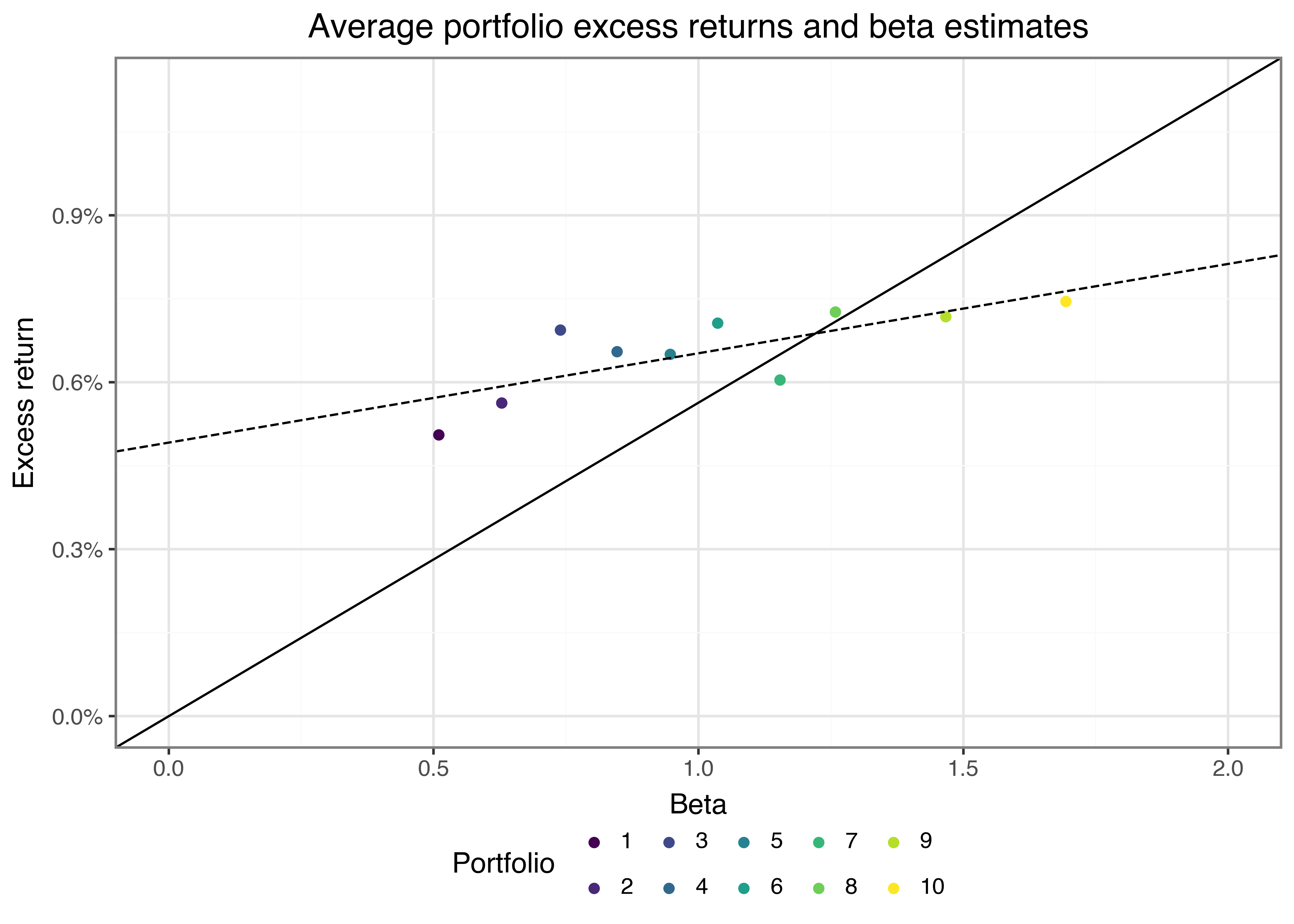
To provide more evidence against the CAPM predictions, we again form a long-short strategy that buys the high-beta portfolio and shorts the low-beta portfolio.
beta_longshort = (beta_portfolios
  .assign(
    portfolio=lambda x: (
      x["portfolio"].apply(
        lambda y: "high" if y == x["portfolio"].max()
        else ("low" if y == x["portfolio"].min()
        else y)
      )
    )
  )
  .query("portfolio in ['low', 'high']")
  .pivot_table(index="date", columns="portfolio", values="ret")
  .assign(long_short=lambda x: x["high"]-x["low"])
  .merge(factors_ff3_monthly, how="left", on="date")
)
Again, the resulting long-short strategy does not exhibit statistically significant returns.
model_fit = (sm.OLS.from_formula(
    formula="long_short ~ 1",
    data=beta_longshort
  )
  .fit(cov_type="HAC", cov_kwds={"maxlags": 1})
)
prettify_result(model_fit)
OLS Model:
long_short ~ 1
Coefficients:
Estimate Std. Error t-Statistic p-Value
Intercept 0.002 0.003 0.75 0.453
Summary statistics:
- Number of observations: 707
- R-squared: -0.000, Adjusted R-squared: -0.000
- F-statistic not available
However, controlling for the effect of beta, the long-short portfolio yields a statistically significant negative CAPM-adjusted alpha, although the average excess stock returns should be zero according to the CAPM. The results thus provide no evidence in support of the CAPM. The negative value has been documented as the so-called betting-against-beta factor (Frazzini and Pedersen 2014). Betting-against-beta corresponds to a strategy that shorts high-beta stocks and takes a (levered) long position in low-beta stocks. If borrowing constraints prevent investors from taking positions on the security market line they are instead incentivized to buy high-beta stocks, which leads to a relatively higher price (and therefore lower expected returns than implied by the CAPM) for such high-beta stocks. As a result, the betting-against-beta strategy earns from providing liquidity to capital-constrained investors with lower risk aversion.
model_fit = (sm.OLS.from_formula(
    formula="long_short ~ 1 + mkt_excess",
    data=beta_longshort
  )
  .fit(cov_type="HAC", cov_kwds={"maxlags": 1})
)
prettify_result(model_fit)
OLS Model:
long_short ~ 1 + mkt_excess
Coefficients:
Estimate Std. Error t-Statistic p-Value
Intercept -0.004 0.002 -1.763 0.078
mkt_excess 1.137 0.069 16.527 0.000
Summary statistics:
- Number of observations: 707
- R-squared: 0.433, Adjusted R-squared: 0.432
- F-statistic: 273.136 on 1 and 705 DF, p-value: 0.000
Figure 3 shows the annual returns of the extreme beta portfolios we are mainly interested in. The figure illustrates no consistent striking patterns over the last years; each portfolio exhibits periods with positive and negative annual returns.
beta_longshort_year = (beta_longshort
  .assign(year=lambda x: x["date"].dt.year)
  .groupby("year")
  .aggregate(
    low=("low", lambda x: (1+x).prod()-1),
    high=("high", lambda x: (1+x).prod()-1),
    long_short=("long_short", lambda x: (1+x).prod()-1)
  )
  .reset_index()
  .melt(id_vars="year", var_name="name", value_name="value")
)

beta_longshort_figure = (
  ggplot(
    beta_longshort_year,
    aes(x="year", y="value", fill="name")
  )
  + geom_col(position="dodge")
  + facet_wrap("~name", ncol=1)
  + labs(x="", y="", title="Annual returns of beta portfolios")
  + scale_y_continuous(labels=percent_format())
  + theme(legend_position="none")
)
beta_longshort_figure.show()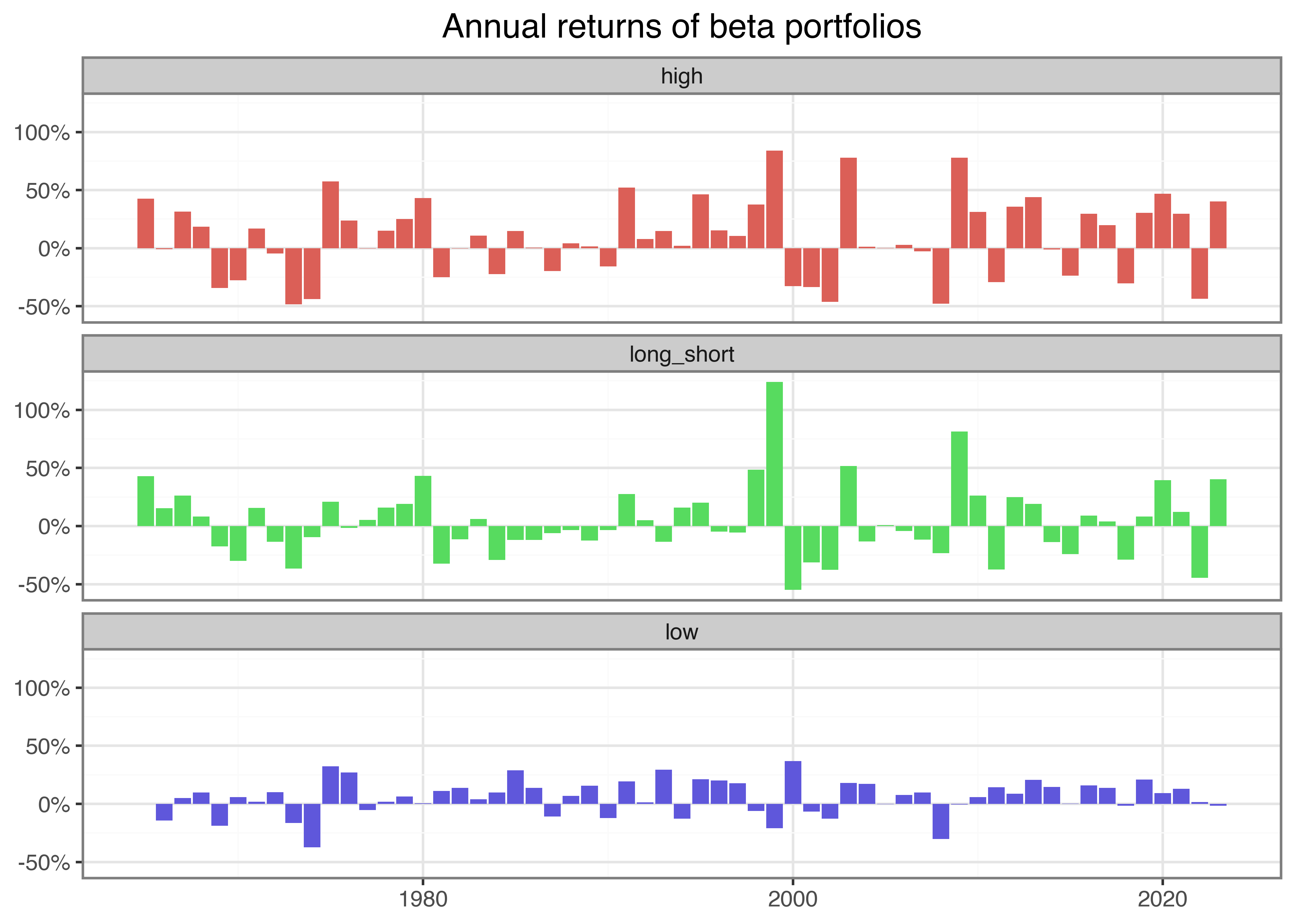
Overall, this chapter shows how functional programming can be leveraged to form an arbitrary number of portfolios using any sorting variable and how to evaluate the performance of the resulting portfolios. In the next chapter, we dive deeper into the many degrees of freedom that arise in the context of portfolio analysis.
Key Takeaways
- Univariate portfolio sorts assess whether a single firm characteristic, like lagged market beta, can predict future excess returns.
- Portfolios are formed each month using quantile breakpoints, with returns computed using value-weighted averages to reflect realistic investment strategies.
- A long-short strategy based on beta-sorted portfolios fails to generate significant positive excess returns, contradicting CAPM predictions that higher beta should yield higher returns.
- The analysis highlights the “betting against beta” anomaly, where low-beta portfolios deliver higher alphas than high-beta portfolios, providing evidence against the CAPM
- The functional programming capabilities of Python enable scalable and flexible portfolio sorting, making it easy to analyze multiple characteristics and portfolio configurations.
Exercises
- Take the two long-short beta strategies based on different numbers of portfolios and compare the returns. Is there a significant difference in returns? How do the Sharpe ratios compare between the strategies? Find one additional portfolio evaluation statistic and compute it.
- We plotted the alphas of the ten beta portfolios above. Write a function that tests these estimates for significance. Which portfolios have significant alphas?
- The analysis here is based on betas from monthly returns. However, we also computed betas from daily returns. Re-run the analysis and point out differences in the results.
- Given the results in this chapter, can you define a long-short strategy that yields positive abnormal returns (i.e., alphas)? Plot the cumulative excess return of your strategy and the market excess return for comparison.
References
Bali, Turan G, Robert F Engle, and Scott Murray. 2016. Empirical asset pricing: The cross section of stock returns. John Wiley & Sons. https://doi.org/10.1002/9781118445112.stat07954.
Frazzini, Andrea, and Lasse Heje Pedersen. 2014. “Betting against beta.” Journal of Financial Economics 111 (1): 1–25. https://doi.org/10.1016/j.jfineco.2013.10.005.
Newey, Whitney K., and Kenneth D. West. 1987. “A simple, positive semi-definite, heteroskedasticity and autocorrelation consistent covariance Matrix.” Econometrica 55 (3): 703–8. http://www.jstor.org/stable/1913610.