Option Pricing via Machine Learning

Note

You are reading Tidy Finance with R. You can find the equivalent chapter for the sibling Tidy Finance with Python here.

This chapter covers machine learning methods in option pricing. First, we briefly introduce regression trees, random forests, and neural networks; these methods are advocated as highly flexible universal approximators, capable of recovering highly non-linear structures in the data. As the focus is on implementation, we leave a thorough treatment of the statistical underpinnings to other textbooks from authors with a real comparative advantage on these issues. We show how to implement random forests and deep neural networks with tidy principles using tidymodels and the torch package for more complicated network structures.

Machine learning (ML) is seen as a part of artificial intelligence. ML algorithms build a model based on training data in order to make predictions or decisions without being explicitly programmed to do so. While ML can be specified along a vast array of different branches, this chapter focuses on so-called supervised learning for regressions. The basic idea of supervised learning algorithms is to build a mathematical model for data that contains both the inputs and the desired outputs. In this chapter, we apply well-known methods such as random forests and neural networks to a simple application in option pricing. More specifically, we create an artificial dataset of option prices for different values based on the Black-Scholes pricing equation for call options. Then, we train different models to learn how to price call options without prior knowledge of the theoretical underpinnings of the famous option pricing equation by Black and Scholes (1973).

Throughout this chapter, we need the following R packages.

library(tidyverse)
library(tidymodels)
library(torch)
library(brulee)
library(hardhat)
library(ranger)
library(glmnet)

The package torch (Falbel et al. 2023) provides functionality to define and train neural networks and is based on PyTorch (Paszke et al. 2019), while brulee (Kuhn and Falbel 2023) provides several basic modeling functions that use the torch infrastructure. The package ranger (Wright and Ziegler 2017) provides a fast implementation for random forests and hardhat (Vaughan and Kuhn 2022) is a helper function to for robust data preprocessing at fit time and prediction time.

Regression Trees and Random Forests

Regression trees are a popular ML approach for incorporating multiway predictor interactions. In Finance, regression trees are gaining popularity, also in the context of asset pricing (see, e.g., Bryzgalova, Pelger, and Zhu 2022). Trees possess a logic that departs markedly from traditional regressions. Trees are designed to find groups of observations that behave similarly to each other. A tree grows in a sequence of steps. At each step, a new branch sorts the data leftover from the preceding step into bins based on one of the predictor variables. This sequential branching slices the space of predictors into partitions and approximates the unknown function \(f(x)\) which yields the relation between the predictors \(x\) and the outcome variable \(y\) with the average value of the outcome variable within each partition. For a more thorough treatment of regression trees, we refer to Coqueret and Guida (2020).

Formally, we partition the predictor space into \(J\) non-overlapping regions, \(R_1, R_2, \ldots, R_J\). For any predictor \(x\) that falls within region \(R_j\), we estimate \(f(x)\) with the average of the training observations, \(\hat y_i\), for which the associated predictor \(x_i\) is also in \(R_j\). Once we select a partition \(x\) to split in order to create the new partitions, we find a predictor \(j\) and value \(s\) that define two new partitions, called \(R_1(j,s)\) and \(R_2(j,s)\), which split our observations in the current partition by asking if \(x_j\) is bigger than \(s\): \[R_1(j,s) = \{x \mid x_j < s\} \mbox{ and } R_2(j,s) = \{x \mid x_j \geq s\}.\] To pick \(j\) and \(s\), we find the pair that minimizes the residual sum of square (RSS): \[\sum_{i:\, x_i \in R_1(j,s)} (y_i - \hat{y}_{R_1})^2 + \sum_{i:\, x_i \in R_2(j,s)} (y_i - \hat{y}_{R_2})^2\] As in Factor Selection via Machine Learning in the context of penalized regressions, the first relevant question is: what are the hyperparameter decisions? Instead of a regularization parameter, trees are fully determined by the number of branches used to generate a partition (sometimes one specifies the minimum number of observations in each final branch instead of the maximum number of branches).

Models with a single tree may suffer from high predictive variance. Random forests address these shortcomings of decision trees. The goal is to improve the predictive performance and reduce instability by averaging multiple decision trees. A forest basically implies creating many regression trees and averaging their predictions. To assure that the individual trees are not the same, we use a bootstrap to induce randomness. More specifically, we build \(B\) decision trees \(T_1, \ldots, T_B\) using the training sample. For that purpose, we randomly select features to be included in the building of each tree. For each observation in the test set, we then form a prediction \(\hat{y} = \frac{1}{B}\sum\limits_{i=1}^B\hat{y}_{T_i}\).

Neural Networks

Roughly speaking, neural networks propagate information from an input layer, through one or multiple hidden layers, to an output layer. While the number of units (neurons) in the input layer is equal to the dimension of the predictors, the output layer usually consists of one neuron (for regression) or multiple neurons for classification. The output layer predicts the future data, similar to the fitted value in a regression analysis. Neural networks have theoretical underpinnings as universal approximators for any smooth predictive association (Hornik 1991). Their complexity, however, ranks neural networks among the least transparent, least interpretable, and most highly parameterized ML tools. In finance, applications of neural networks can be found in many different contexts, e.g., Avramov, Cheng, and Metzker (2022), Chen, Pelger, and Zhu (2023), and Gu, Kelly, and Xiu (2020).

Each neuron applies a non-linear activation function \(f\) to its aggregated signal before sending its output to the next layer \[x_k^l = f\left(\theta^k_{0} + \sum\limits_{j = 1}^{N ^l}z_j\theta_{l,j}^k\right)\] Here, \(\theta\) are the parameters to fit, \(N^l\) denotes the number of units (a hyperparameter to tune), and \(z_j\) are the input variables which can be either the raw data or, in the case of multiple chained layers, the outcome from a previous layer \(z_j = x_k-1\). While the easiest case with \(f(x) = \alpha + \beta x\) resembles linear regression, typical activation functions are sigmoid (i.e., \(f(x) = (1+e^{-x})^{-1}\)) or ReLu (i.e., \(f(x) = max(x, 0)\)).

Neural networks gain their flexibility from chaining multiple layers together. Naturally, this imposes many degrees of freedom on the network architecture for which no clear theoretical guidance exists. The specification of a neural network requires, at a minimum, a stance on depth (number of hidden layers), the activation function, the number of neurons, the connection structure of the units (dense or sparse), and the application of regularization techniques to avoid overfitting. Finally, learning means to choose optimal parameters relying on numerical optimization, which often requires specifying an appropriate learning rate. Despite these computational challenges, implementation in R is not tedious at all because we can use the API to torch.

Option Pricing

To apply ML methods in a relevant field of finance, we focus on option pricing. The application in its core is taken from Hull (2020). In its most basic form, call options give the owner the right but not the obligation to buy a specific stock (the underlying) at a specific price (the strike price \(K\)) at a specific date (the exercise date \(T\)). The Black–Scholes price (Black and Scholes 1973) of a call option for a non-dividend-paying underlying stock is given by \[ \begin{aligned} C(S, T) &= \Phi(d_1)S - \Phi(d_1 - \sigma\sqrt{T})Ke^{-r T} \\ d_1 &= \frac{1}{\sigma\sqrt{T}}\left(\ln\left(\frac{S}{K}\right) + \left(r_f + \frac{\sigma^2}{2}\right)T\right) \end{aligned} \] where \(C(S, T)\) is the price of the option as a function of today’s stock price of the underlying, \(S\), with time to maturity \(T\), \(r_f\) is the risk-free interest rate, and \(\sigma\) is the volatility of the underlying stock return. \(\Phi\) is the cumulative distribution function of a standard normal random variable.

The Black-Scholes equation provides a way to compute the arbitrage-free price of a call option once the parameters \(S, K, r_f, T\), and \(\sigma\) are specified (arguably, in a realistic context, all parameters are easy to specify except for \(\sigma\) which has to be estimated). A simple R function allows computing the price as we do below.

black_scholes_price <- function(S, K = 70, r = 0, T = 1, sigma = 0.2) {
  
  d1 <- (log(S / K) + (r + sigma^2 / 2) * T) / (sigma * sqrt(T))
  d2 <- d1 - sigma * sqrt(T)
  price <- S * pnorm(d1) - K * exp(-r * T) * pnorm(d2)
  
  return(price)
}

Learning Black-Scholes

We illustrate the concept of ML by showing how ML methods learn the Black-Scholes equation after observing some different specifications and corresponding prices without us revealing the exact pricing equation.

Data simulation

To that end, we start with simulated data. We compute option prices for call options for a grid of different combinations of times to maturity (T), risk-free rates (r), volatilities (sigma), strike prices (K), and current stock prices (S). In the code below, we add an idiosyncratic error term to each observation such that the prices considered do not exactly reflect the values implied by the Black-Scholes equation.

In order to keep the analysis reproducible, we use set.seed(). A random seed specifies the start point when a computer generates a random number sequence and ensures that our simulated data is the same across different machines.

set.seed(420)

option_prices <- expand_grid(
  S = 40:60,
  K = 20:90,
  r = seq(from = 0, to = 0.05, by = 0.01),
  T = seq(from = 3 / 12, to = 2, by = 1 / 12),
  sigma = seq(from = 0.1, to = 0.8, by = 0.1)
) |>
  mutate(
    black_scholes = black_scholes_price(S, K, r, T, sigma),
    observed_price = map_dbl(
      black_scholes,
      function(x) x + rnorm(1, sd = 0.15)
    )
  )

The code above generates more than 1.5 million random parameter constellations. For each of these values, two observed prices reflecting the Black-Scholes prices are given and a random innovation term pollutes the observed prices. The intuition of this application is simple: the simulated data provides many observations of option prices - by using the Black-Scholes equation we can evaluate the actual predictive performance of a ML method, which would be hard in a realistic context were the actual arbitrage-free price would be unknown.

Next, we split the data into a training set (which contains 1% of all the observed option prices) and a test set that will only be used for the final evaluation. Note that the entire grid of possible combinations contains 1574496 different specifications. Thus, the sample to learn the Black-Scholes price contains only 31,489 observations and is therefore relatively small.

split <- initial_split(option_prices, prop = 1 / 100)

We process the training dataset further before we fit the different ML models. We define a recipe() that defines all processing steps for that purpose. For our specific case, we want to explain the observed price by the five variables that enter the Black-Scholes equation. The true prices (stored in column black_scholes) should obviously not be used to fit the model. The recipe also reflects that we standardize all predictors to ensure that each variable exhibits a sample average of zero and a sample standard deviation of one.

rec <- recipe(observed_price ~ .,
  data = option_prices
) |>
  step_rm(black_scholes) |>
  step_normalize(all_predictors())

Single layer networks and random forests

Next, we show how to fit a neural network to the data. Note that this requires that torch is installed on your local machine. The function mlp() from the package parsnip provides the functionality to initialize a single layer, feed-forward neural network. The specification below defines a single layer feed-forward neural network with 10 hidden units. We set the number of training iterations to epochs = 500. The option set_mode("regression") specifies a linear activation function for the output layer.

nnet_model <- mlp(
  epochs = 500,
  hidden_units = 10,
  activation = "sigmoid",
  penalty = 0.0001
) |>
  set_mode("regression") |>
  set_engine("brulee", verbose = FALSE)

The verbose = FALSE argument prevents logging the results to the console. We can follow the straightforward tidymodel workflow as in Factor Selection via Machine Learning: define a workflow, equip it with the recipe, and specify the associated model. Finally, fit the model with the training data.

nn_fit <- workflow() |>
  add_recipe(rec) |>
  add_model(nnet_model) |>
  fit(data = training(split))

Once you are familiar with the tidymodels workflow, it is a piece of cake to fit other models from the parsnip family. For instance, the model below initializes a random forest with 50 trees contained in the ensemble, where we require at least 2000 observations in a node. The random forests are trained using the package ranger, which is required to be installed in order to run the code below.

rf_model <- rand_forest(
  trees = 50,
  min_n = 2000
) |>
  set_engine("ranger") |>
  set_mode("regression")

Fitting the model follows exactly the same convention as for the neural network before.

rf_fit <- workflow() |>
  add_recipe(rec) |>
  add_model(rf_model) |>
  fit(data = training(split))

Deep neural networks

A deep neural network is a neural network with multiple layers between the input and output layers. By chaining multiple layers together, more complex structures can be represented with fewer parameters than simple shallow (one-layer) networks as the one implemented above. For instance, image or text recognition are typical tasks where deep neural networks are used (for applications of deep neural networks in finance, see, for instance, Jiang, Kelly, and Xiu 2023; Jensen et al. 2022).

Note that while the tidymodels workflow is extremely convenient, these more sophisticated multi-layer (so-called deep) neural networks are not supported by tidymodels yet (as of September 2022). Instead, an implementation of a deep neural network in R requires additional computational tools. For that reason, the code snippet below illustrates how to initialize a sequential model with three hidden layers ith 10 units per layer. The brulee package provides a convenient interface to torch and is flexible enough to handle different activation functions.

deep_nnet_model <- mlp(
  epochs = 500,
  hidden_units = c(10, 10, 10),
  activation = "sigmoid",
  penalty = 0.0001
) |>
  set_mode("regression") |>
  set_engine("brulee", verbose = FALSE)

To train the neural network, we provide the inputs (x) and the variable to predict (y) and then fit the parameters. Note the slightly tedious use of the method extract_mold(nn_fit). Instead of simply using the raw data, we fit the neural network with the same processed data that is used for the single-layer feed-forward network. What is the difference to simply calling x = training(data) |> select(-observed_price, -black_scholes)? Recall that the recipe standardizes the variables such that all columns have unit standard deviation and zero mean. Further, it adds consistency if we ensure that all models are trained using the same recipe such that a change in the recipe is reflected in the performance of any model. A final note on a potentially irritating observation: fit() alters the model - this is one of the few instances, where a function in R alters the input such that after the function call the object model is not same anymore!

deep_nn_fit <- workflow() |>
  add_recipe(rec) |>
  add_model(deep_nnet_model) |>
  fit(data = training(split))

Universal approximation

Before we evaluate the results, we implement one more model. In principle, any non-linear function can also be approximated by a linear model containing the input variables’ polynomial expansions. To illustrate this, we first define a new recipe, rec_linear, which processes the training data even further. We include polynomials up to the fifth degree of each predictor and then add all possible pairwise interaction terms. The final recipe step, step_lincomb(), removes potentially redundant variables (for instance, the interaction between \(r^2\) and \(r^3\) is the same as the term \(r^5\)). We fit a Lasso regression model with a pre-specified penalty term (consult Factor Selection via Machine Learning on how to tune the model hyperparameters).

rec_linear <- rec |>
  step_poly(all_predictors(),
    degree = 5,
    options = list(raw = TRUE)
  ) |>
  step_interact(terms = ~ all_predictors():all_predictors()) |>
  step_lincomb(all_predictors())

lm_model <- linear_reg(penalty = 0.01) |>
  set_engine("glmnet")

lm_fit <- workflow() |>
  add_recipe(rec_linear) |>
  add_model(lm_model) |>
  fit(data = training(split))

Prediction Evaluation

Finally, we collect all predictions to compare the out-of-sample prediction error evaluated on 10,000 new data points. Note that for the evaluation, we use the call to extract_mold() to ensure that we use the same pre-processing steps for the testing data across each model. We also use the somewhat advanced functionality in forge(), which provides an easy, consistent, and robust pre-processor at prediction time.

out_of_sample_data <- testing(split) |>
  slice_sample(n = 10000)

predictive_performance <- deep_nn_fit |>
  predict(out_of_sample_data)|>
  rename("Deep NN" = .pred) |>
  bind_cols(nn_fit |>
    predict(out_of_sample_data)) |>
  rename("Single layer" = .pred) |>
  bind_cols(lm_fit |> predict(out_of_sample_data)) |>
  rename("Lasso" = .pred) |>
  bind_cols(rf_fit |> predict(out_of_sample_data)) |>
  rename("Random forest" = .pred) |>
  bind_cols(out_of_sample_data) |>
  pivot_longer("Deep NN":"Random forest", names_to = "Model") |>
  mutate(
    moneyness = (S - K),
    pricing_error = abs(value - black_scholes)
  )

In the lines above, we use each of the fitted models to generate predictions for the entire test dataset of option prices. We evaluate the absolute pricing error as one possible measure of pricing accuracy, defined as the absolute value of the difference between predicted option price and the theoretical correct option price from the Black-Scholes model. We show the results graphically in Figure 1.

predictive_performance |>
  ggplot(aes(
    x = moneyness, 
    y = pricing_error, 
    color = Model,
    linetype = Model
    )) +
  geom_jitter(alpha = 0.05) +
  geom_smooth(se = FALSE, method = "gam", formula = y ~ s(x, bs = "cs")) +
  facet_wrap(~Model, ncol = 2) + 
  labs(
    x = "Moneyness (S - K)", color = NULL,
    y = "Absolut prediction error (USD)",
    title = "Prediction errors of call option prices for different models",
    linetype = NULL
  )

Figure 1: Absolut prediction error in USD for the different fitted methods. The prediction error is evaluated on a sample of call options that were not used for training.

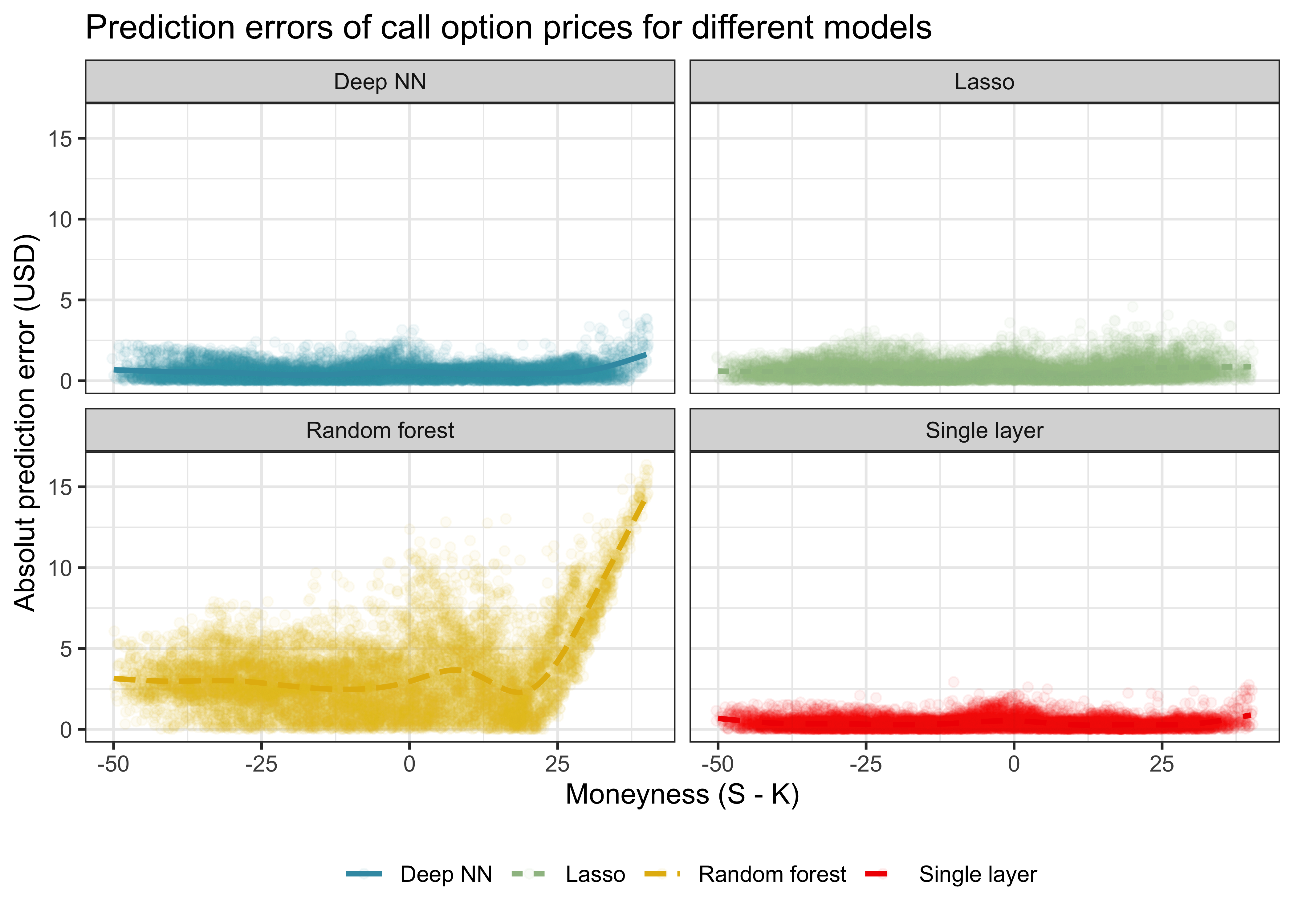
The results can be summarized as follows:

1. All ML methods seem to be able to price call options after observing the training test set.
2. The average prediction errors increase for far in-the-money options.
3. Random forest and the Lasso seem to perform consistently worse in predicting option prices than the neural networks.
4. The complexity of the deep neural network relative to the single-layer neural network does not result in better out-of-sample predictions.

Key Takeaways

• Machine learning methods like random forests and neural networks can be used to estimate call option prices in R without relying on the Black-Scholes formula.
• Simulating noisy option price data and applying supervised learning models via the tidymodels framework provides a clean, reproducible analysis.
• Deep neural networks do not consistently outperform single-layer networks, underscoring the trade-off between model complexity and prediction performance.

Exercises

1. Write a function that takes y and a matrix of predictors X as inputs and returns a characterization of the relevant parameters of a regression tree with 1 branch.
2. Create a function that creates predictions for a new matrix of predictors newX based on the estimated regression tree.
3. Use the package rpart to grow a tree based on the training data and use the illustration tools in rpart to understand which characteristics the tree deems relevant for option pricing.
4. Make use of a training and a test set to choose the optimal depth (number of sample splits) of the tree.
5. Use brulee to initialize a sequential neural network that can take the predictors from the training dataset as input, contains at least one hidden layer, and generates continuous predictions. This sounds harder than it is: see a simple regression example here. How many parameters does the neural network you aim to fit have?
6. Compile the object from the previous exercise. It is important that you specify a loss function. Illustrate the difference in predictive accuracy for different architecture choices.

References

Avramov, Doron, Si Cheng, and Lior Metzker. 2022. “Machine learning vs. economic restrictions: Evidence from stock return predictability.” Management Science 69 (5): 2547–3155. http://dx.doi.org/10.2139/ssrn.3450322.

Black, Fischer, and Myron Scholes. 1973. “The pricing of options and corporate liabilities.” Journal of Political Economy 81 (3): 637–54. https://www.jstor.org/stable/1831029.

Bryzgalova, Svetlana, Markus Pelger, and Jason Zhu. 2022. “Forest through the trees: Building cross-sections of stock returns.” Working Paper. http://dx.doi.org/10.2139/ssrn.3493458.

Chen, Luyang, Markus Pelger, and Jason Zhu. 2023. “Deep learning in asset pricing.” Management Science. https://doi.org/10.48550/arXiv.1904.00745.

Coqueret, Guillaume, and Tony Guida. 2020. Machine learning for factor investing: R version. Chapman; Hall/CRC. https://www.mlfactor.com/.

Falbel, Daniel, Javier Luraschi, Dmitriy Selivanov, Athos Damiani, Christophe Regouby, Krzysztof Joachimiak, and Hamada S. Badr. 2023. torch: Tensors and Neural Networks with ’GPU’ Acceleration. https://CRAN.R-project.org/package=torch.

Gu, Shihao, Bryan Kelly, and Dacheng Xiu. 2020. “Empirical asset pricing via machine learning.” Edited by Andrew Karolyi. Review of Financial Studies 33 (5): 2223–73. https://doi.org/10.1093/rfs/hhaa009.

Hornik, Kurt. 1991. “Approximation capabilities of multilayer feedforward networks.” Neural Networks 4 (2): 251–57. https://doi.org/10.1016/0893-6080(91)90009-T.

Hull, John C. 2020. Machine learning in business. An introduction to the world of data science. Independently published.

Jensen, Theis Ingerslev, Bryan T. Kelly, Semyon Malamud, and Lasse Heje Pedersen. 2022. “Machine Learning and the Implementable Efficient Frontier.” Working Paper. https://doi.org/10.2139/ssrn.3491942.

Jiang, Jingwen, Bryan T. Kelly, and Dacheng Xiu. 2023. “(Re-)Imag(in)ing Price Trends.” The Journal of Finance 78 (6): 3193–3249. https://doi.org/10.1111/jofi.13268.

Kuhn, Max, and Daniel Falbel. 2023. brulee: High-Level Modeling Functions with ’torch’. https://CRAN.R-project.org/package=brulee.

Paszke, Adam, Sam Gross, Francisco Massa, Adam Lerer, James Bradbury, Gregory Chanan, Trevor Killeen, et al. 2019. “PyTorch: An Imperative Style, High-Performance Deep Learning Library.” In Advances in Neural Information Processing Systems 32, 8024–35. Curran Associates, Inc. http://papers.neurips.cc/paper/9015-pytorch-an-imperative-style-high-performance-deep-learning-library.pdf.

Vaughan, Davis, and Max Kuhn. 2022. hardhat: Construct modeling packages. https://CRAN.R-project.org/package=hardhat.

Wright, Marvin N., and Andreas Ziegler. 2017. “ranger: A fast implementation of random forests for high dimensional data in C++ and R.” Journal of Statistical Software 77 (1): 1–17. http://dx.doi.org/10.18637/jss.v077.i01.