Fast Portfolio Sorts

Implementing standard tasks like portfolio sorts in R can be approached in various ways, including using base R, dplyr, or data.table. For researchers and data analysts, it’s crucial that these implementations are both correct and efficient. Even though portfolio sorting is a relatively simple task, the need to sort portfolios in numerous ways due to the variety of sorting variables and methodological uncertainties can make computational efficiency critical. This blog post will benchmark the performance of different sorting methods in R, focusing on execution time, to provide insights for data analysts and portfolio managers on choosing the most efficient approach.

We’ll dive into the following sorting approaches:

• Use the built-in base functions that ship with every R installation.
• Leverage the popular dplyr package and workhorse of Tidy Finance with R.
• Explore the powerful data.table package using on-the-fly column creation.
• Compare to the data.table variant with in-place mutations.
• Combine the dplyr syntax with data.table’s performance through dtplyr.

Throughout this blog post, I’ll use the following packages. Notably, bench is used to create benchmarking results.

library(dplyr)
library(dtplyr)
library(data.table)
library(bench)
library(purrr)
library(RSQLite)
library(ggplot2)

Data preparation

First, I start by loading the monthly CRSP data from our database (see WRDS, CRSP, and Compustat for details). The dataset has about 3 million rows and contains monthly returns between 1960 and 2023 for about 26,000 stocks. I also make sure that the data comes as a tibble for dplyr, a data.frame for base, two data.tables for the two data.table approaches, and a ‘lazy’ data table for dtplyr because I want to avoid any conversion issues in the portfolio assignments.

tidy_finance <- dbConnect(
  SQLite(),
  "../../data/tidy_finance_r.sqlite",
  extended_types = TRUE
)

crsp_monthly_dplyr <- tbl(tidy_finance, "crsp_monthly") |>
  select(permno, month, ret_excess, mktcap_lag) |>
  collect()

crsp_monthly_base <- as.data.frame(crsp_monthly_dplyr)

crsp_monthly_dt <- copy(as.data.table(crsp_monthly_dplyr))

crsp_monthly_dtip <- copy(as.data.table(crsp_monthly_dplyr))

crsp_monthly_dtplyr <- lazy_dt(copy(crsp_monthly_dt))

Note data.table in R uses reference semantics, which means that modifying one data.table object could potentially modify another if they share the same underlying data. Therefore, copy() ensures that crsp_monthly_dt is an independent copy of the data, preventing unintentional side effects from modifications in subsequent operations and ensuring a fair comparison.

Defining portfolio sorts

As a common denominator across approaches, I introduce a stripped down version of assign_portfolio() that can also be found in the tidyfinance package.

assign_portfolio <- function(data, sorting_variable, n_portfolios) {
  
  breakpoints <- quantile(
    data[[sorting_variable]], 
    probs = seq(0, 1, length.out = n_portfolios + 1), 
    na.rm = TRUE, names = FALSE
  )

  findInterval(
    data[[sorting_variable]], breakpoints, all.inside = TRUE
  )
}

The goal is to apply this function to the cross-section of stocks in each month and then compute average excess returns for each portfolio across all months.

If we want to apply the function above to each month using only base, then we have to first split the data.frame into multiple parts and lapply() the function to each part. After we combined the parts again to one big data.frame, we can use aggregate() to compute the average excess returns.

sort_base <- function() {
  crsp_monthly_base$portfolio <- with(
    crsp_monthly_base, 
    ave(mktcap_lag, month, FUN = function(x) assign_portfolio(data.frame(mktcap_lag = x), "mktcap_lag", n_portfolios = 10))
  )
  
  mean_ret_excess <- with(
    crsp_monthly_base, 
    tapply(ret_excess, portfolio, mean)
  )

  data.frame(
    portfolio = names(mean_ret_excess), 
    ret = unlist(mean_ret_excess)
  )
}
bench::system_time(sort_base())

process    real 
  3.08s   3.04s 

This approach takes about 3 seconds per execution on my machine and is in fact more than 8-times slower than the other approaches! To create a more nuanced picture for the fast and arguably more interesting approaches, I’ll drop the base approach going forward.

If we want to perform the same logic using dplyr, we can use the following approach. Note that I use as.data.frame() for all approaches to ensure that the output format is the same for all approaches - a necessary requirement for a meaningful benchmark (otherwise code would not be equivalent).

sort_dplyr <- function() {
  crsp_monthly_dplyr |> 
    group_by(month) |> 
    mutate(
      portfolio = assign_portfolio(
        pick(everything()), "mktcap_lag", n_portfolios = 10),
      by = "month"
    ) |> 
    group_by(portfolio) |> 
    summarize(ret = mean(ret_excess)) |> 
    as.data.frame()
}
sort_dplyr()

   portfolio     ret
1          1 0.02270
2          2 0.00512
3          3 0.00482
4          4 0.00515
5          5 0.00548
6          6 0.00608
7          7 0.00637
8          8 0.00680
9          9 0.00647
10        10 0.00579

The equivalent approach in data.table looks as follows. Note that I deliberately don’t use any pipe or intermediate assignments as to avoid any performance overhead that these might introduce. I also avoid using the in-place modifier := because it would create a new permanent column in crsp_monthly_dt, which I don’t need for the on-the-fly aggregation and it also doesn’t happen in dplyr.

sort_dt <- function() {
  as.data.frame(crsp_monthly_dt[
    , .(portfolio = assign_portfolio(.SD, "mktcap_lag", n_portfolios = 10), month, ret_excess), by = .(month)][
      , .(ret = mean(ret_excess)), keyby = .(portfolio)
      ])
}
sort_dt()

   portfolio     ret
1          1 0.02270
2          2 0.00512
3          3 0.00482
4          4 0.00515
5          5 0.00548
6          6 0.00608
7          7 0.00637
8          8 0.00680
9          9 0.00647
10        10 0.00579

However, as the performance benefit of data.table may manifest itself through its in-place modification capabilties, I also introduce a second version of the data.table expression. Note that in this version crsp_monthly_dtip gets a permanent column portfolio that is overwritten in each iteration.

sort_dtip <- function() {
  as.data.frame(crsp_monthly_dtip[
    , portfolio := assign_portfolio(.SD, "mktcap_lag", n_portfolios = 10), by = .(month)][
      , .(ret = mean(ret_excess)), keyby = .(portfolio)
      ])
}
sort_dtip()

   portfolio     ret
1          1 0.02270
2          2 0.00512
3          3 0.00482
4          4 0.00515
5          5 0.00548
6          6 0.00608
7          7 0.00637
8          8 0.00680
9          9 0.00647
10        10 0.00579

Lastly, I add the dtplyr implementation that also takes a data.table as input and internally converts dplyr code to data.table syntax. Note that the final as.data.frame() call is used to access the results and ensure that the result format is consistent with the other approaches.

sort_dtplyr <- function() {
  crsp_monthly_dtplyr |> 
    group_by(month) |> 
    mutate(
      portfolio = assign_portfolio(
        pick(everything()), "mktcap_lag", n_portfolios = 10),
      by = "month"
    )  |> 
    group_by(portfolio) |> 
    summarize(ret = mean(ret_excess, na.rm = TRUE)) |> 
    as.data.frame()
}
sort_dtplyr()

   portfolio     ret
1          1 0.02270
2          2 0.00512
3          3 0.00482
4          4 0.00515
5          5 0.00548
6          6 0.00608
7          7 0.00637
8          8 0.00680
9          9 0.00647
10        10 0.00579

Now that we have verified that all code chunks create the same average excess returns per portfolio, we can proceed to the performance evaluation.

Benchmarking results

The bench package is a great utility for benchmarking and timing expressions in R. It provides functions that allow you to measure the execution time of expressions or code chunks. This can be useful for comparing the performance of different approaches or implementations, or for identifying potential bottlenecks in your code. The following code evaluates each approach from above a 100 times and collects the results.

iterations <- 100

results <- bench::mark(
  sort_dplyr(), sort_dt(), sort_dtip(), sort_dtplyr(), 
  iterations = iterations
)

The following plot shows the distributions of execution times as violin plots. You can see that dplyr takes the lead and is followed closely by both data.table variants, while dtplyr takes the third place.

autoplot(results, type = "violin") +
  labs(y = NULL, x = NULL, 
       title = "Execution time of porfolio sorts using dplyr, data.table, and dtplyr",
       subtitle = "'dt' refers to data.table without in-place modification and 'dtip' with in-place modification")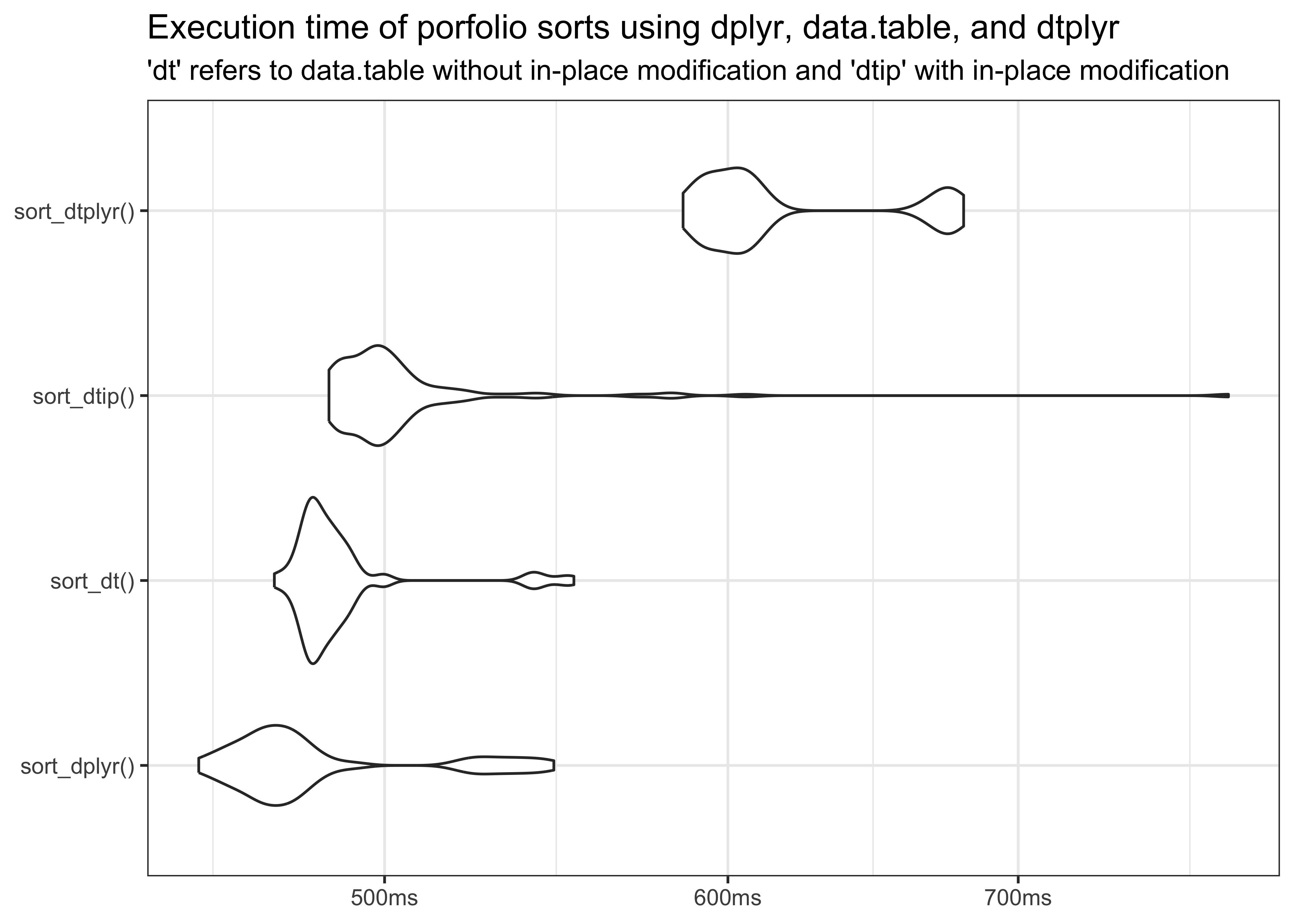

Note that all three methods are quite fast and take less than 1 second, given that the task is to assign 10 portfolios across up to 26,000 stocks for 755 months. In fact, dplyr yields the fastest execution times, followed by both data.table implementations and dtplyr.

Why is data.table slower than dplyr? It is generally believed that data.table is faster than dplyr for data manipulation tasks. The example above shows that it actually depends on the application. On the one hand, the data set might be ‘too small’ for the performance benefits of data.table to kick in. On the other hand, sorting the portfolios using the assign_portfolio() function might be better suited for the dplyr execution backend than the data.table backend.

Why is dtplyr slower than data.table? On the one hand, dtplyr translates dplyr operations into data.table syntax. This translation process introduces some overhead, as dtplyr needs to interpret the dplyr code and convert it into equivalent data.table operations. On the other hand, dtplyr does not modify in place by default, so it typcially makes a copy that would not be necessary if you were using data.table directly.

Concluding remarks

The key takeway is that neither of the libraries is strictly more efficient than the other. If you really search for performance among R libraries, you have to carefully choose a library for your specific application and think hard about optimizing the logic of your code to the chosen library.

If you have ideas how to optimize any of the approaches, please reach out to us! In particular, we’d love to optimize base sufficiently for it to be included in the benchmark tests.