Financial Statement Analysis

Financial statements and ratios are fundamental tools for understanding and evaluating companies. While we discuss how assets are priced in equilibrium in the previous chapter on the Capital Asset Pricing Model, this chapter examines how investors and analysts assess companies using accounting information. Financial statements serve as the primary source of standardized information about a company’s operations, financial position, and performance. Their standardization and legal requirements make them particularly valuable as all companies must file financial statements.

Building on this standardized information, financial ratios transform raw accounting data into meaningful metrics that facilitate analysis across companies and over time. These ratios serve multiple purposes in both academic research and practical applications. They enable investors to benchmark companies against their peers, identify industry trends, and screen for investment opportunities. In academic finance, ratios play a crucial role in asset pricing models (e.g., the book-to-market ratio in the Fama-French three-factor model) and corporate finance (e.g., capital structure research). In many practical applications, ratios help assess a company’s financial health and performance.

This chapter demonstrates how to access, process, and analyze financial statements. We start by reviewing the financial statements balance sheet, income statement, and cash flow statement. Then, we download publicly available statements to calculate key financial ratios, implement common screening strategies, and evaluate companies. Our analysis combines theoretical frameworks with practical implementation, providing tools for both academic research and investment practice.

For the purpose of this chapter, we use financial statements provided by the US Securities and Exchange Commission (i.e., SEC). While the SEC provides a web interface to search filings, programmatic access to financial statements greatly facilitates systematic analyses such as ours. The Financial Modeling Prep (FMP) API offers such programmatic access, which we can leverage through the fmpapi package.

The FMP API’s free tier provides access to:

250 API calls per day,
Five years of historical fundamental data,
Real-time and historical stock prices, and
Key financial ratios and metrics.

Tip

The fmpapi package is developed by Christoph Scheuch and not sponsored by or affiliated with FMP. However, you can get 15% off your FMP subscription by using this affiliate link. By signing up through this link, you also support the development of this package at no extra cost to you.

Next to fmpapi, we use the following packages throughout this chapter:

library(tidyverse)
library(tidyfinance)
library(scales)
library(ggrepel)
library(fmpapi)

theme_set(theme_minimal())

import polars as pl

from dotenv import load_dotenv
from fmpapi import fmp_get
from plotnine import *
from mizani.formatters import percent_format
from adjustText import adjust_text

load_dotenv()

True

theme_set(theme_minimal())

By default, fmp_get() returns a polars data frame, so we can work with the results directly.

Balance Sheet Statements

The balance sheet is one of the three primary financial statements capturing a company’s financial position at a specific moment in time. The statement lists all uses (assets) and sources (liabilities and equity) of funds, which result in the fundamental accounting equation:

\[\text{Assets} = \text{Liabilities} + \text{Equity}\]

This equation reflects a core principle of accounting: a company’s resources (assets) must equal its sources of funding, whether from creditors (liabilities) or investors (shareholders’ equity). Assets represent resources that the company controls and expects to generate future economic benefits, such as cash, inventory, or equipment. Liabilities encompass all obligations to external parties, from short-term payables to long-term debt. Shareholders’ equity represents the residual claim on assets after accounting for all liabilities.

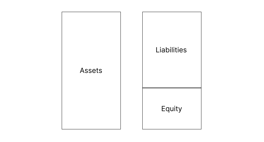
Figure 1 provides a stylized representation of a balance sheet’s structure. The visualization highlights how assets on the left side must equal the combined claims of creditors and shareholders on the right side.

Figure 1: A stylized representation of a balance sheet statement.

The asset side of the balance sheet typically comprises three main categories, each serving different roles in the company’s operations:

Current assets: These are assets expected to be converted into cash or used within one operating cycle (typically one year). They include, e.g., cash and cash equivalents, short-term investments, accounts receivable (money owed by customers), and inventory (raw materials, work in progress, and finished goods).
Non-current assets: These long-term assets support the company’s operations beyond one year, e.g., property, plant, and equipment (PP&E), long-term investments, and other long-term assets.
Intangible assets: These non-physical assets often represent significant value in modern companies, e.g., patents and intellectual property, trademarks and brands, and goodwill from acquisitions (a premium paid on the book value of the acquired assets). Intangible assets are usually also considered long-term assets, which means that they are included in the group of non-current assets.

Figure 2 illustrates this breakdown of assets, showing how companies classify their resources.

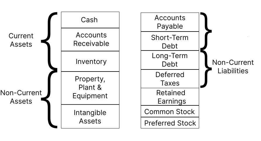
Figure 2: A stylized representation of a balance sheet breakdown.

Figure 2 also shows the breakdown of liabilities. The liability side similarly follows a temporal classification, dividing obligations based on when they come due:

Current liabilities: Obligations due within one year such as accounts payable, short-term debt, current portion of long-term debt, and accrued expenses.
Non-current liabilities: Long-term obligations such as long-term debt, bonds payable, deferred tax liabilities, and pension obligations.

Lastly, the equity section represents ownership claims and typically consists of:

Retained earnings: Accumulated profits reinvested in the business.
Common stock: Par value and additional paid-in capital from share issuance.
Preferred stock: Hybrid securities with characteristics of both debt and equity.

Figure 2 also depicts this equity structure, showing how companies track different forms of ownership claims.

To illustrate these concepts in practice, Figure 3 presents Microsoft’s balance sheet from 2023. This real-world example demonstrates how one of the world’s largest technology companies structures its financial position, reflecting both traditional elements like PP&E and modern aspects like significant intangible assets.

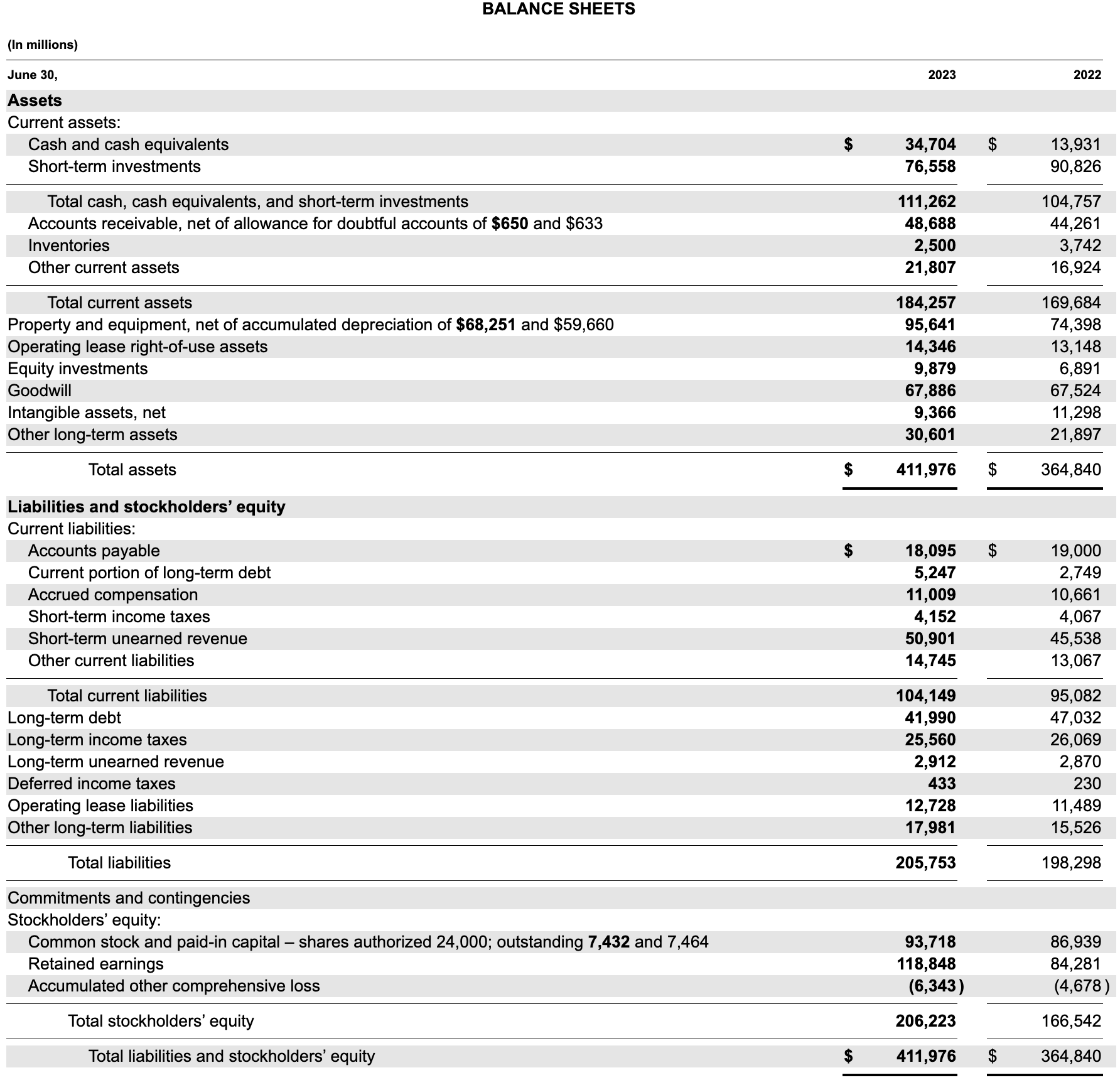
Figure 3: A screenshot of the balance sheet statement of Microsoft in 2023.

While there are more details, the basic structure is exactly the same as in the introduction above. Importantly, the balance sheet obeys the fundamental accounting equation as assets are equal to the sum of liabilities and equity. In subsequent sections, we will explore how to analyze such statements using financial ratios, particularly focusing on measures of liquidity, solvency, and efficiency.

Let us examine Microsoft’s balance sheet statements using the fmp_get() function. This function requires three main arguments: The type of financial data to retrieve (resource), the stock ticker symbol (symbol), and additional parameters like periodicity and number of periods (params).

fmp_get(
  resource = "balance-sheet-statement",
  symbol = "MSFT",
  params = list(period = "annual", limit = 5)
)

# A tibble: 5 × 61
  date       symbol reported_currency cik        filing_date
  <date>     <chr>  <chr>             <chr>      <date>     
1 2025-06-30 MSFT   USD               0000789019 2025-07-30 
2 2024-06-30 MSFT   USD               0000789019 2024-07-30 
3 2023-06-30 MSFT   USD               0000789019 2023-07-27 
4 2022-06-30 MSFT   USD               0000789019 2022-07-28 
5 2021-06-30 MSFT   USD               0000789019 2021-07-29 
# ℹ 56 more variables: accepted_date <dttm>, fiscal_year <chr>,
#   period <chr>, cash_and_cash_equivalents <dbl>,
#   short_term_investments <dbl>,
#   cash_and_short_term_investments <dbl>, net_receivables <dbl>,
#   accounts_receivables <dbl>, other_receivables <int>,
#   inventory <dbl>, prepaids <int>, other_current_assets <dbl>,
#   total_current_assets <dbl>, …

fmp_get(
  resource="balance-sheet-statement",
  symbol="MSFT",
  params={"period": "annual", "limit": 5}
)

shape: (5, 61)

date	symbol	reported_currency	cik	filing_date	accepted_date	fiscal_year	period	cash_and_cash_equivalents	short_term_investments	cash_and_short_term_investments	net_receivables	accounts_receivables	other_receivables	inventory	prepaids	other_current_assets	total_current_assets	property_plant_equipment_net	goodwill	intangible_assets	goodwill_and_intangible_assets	long_term_investments	tax_assets	other_non_current_assets	total_non_current_assets	other_assets	total_assets	total_payables	account_payables	other_payables	accrued_expenses	short_term_debt	capital_lease_obligations_current	tax_payables	deferred_revenue	other_current_liabilities	total_current_liabilities	long_term_debt	capital_lease_obligations_non_current	deferred_revenue_non_current	deferred_tax_liabilities_non_current	other_non_current_liabilities	total_non_current_liabilities	other_liabilities	capital_lease_obligations	total_liabilities	treasury_stock	preferred_stock	common_stock	retained_earnings	additional_paid_in_capital	accumulated_other_comprehensive_income_loss	other_total_stockholders_equity	total_stockholders_equity	total_equity	minority_interest	total_liabilities_and_total_equity	total_investments	total_debt	net_debt
date	str	str	str	date	datetime[μs]	i32	str	i64	i64	i64	i64	i64	i64	i64	i64	i64	i64	i64	i64	i64	i64	i64	i64	i64	i64	i64	i64	i64	i64	i64	i64	i64	i64	i64	i64	i64	i64	i64	i64	i64	i64	i64	i64	i64	i64	i64	i64	i64	i64	i64	i64	i64	i64	i64	i64	i64	i64	i64	i64	i64
2025-06-30	"MSFT"	"USD"	"0000789019"	2025-07-30	2025-07-30 16:11:40	2025	"FY"	30242000000	64313000000	94555000000	69905000000	69905000000	0	938000000	0	25733000000	191131000000	229789000000	119509000000	22604000000	142113000000	15133000000	0	40837000000	427872000000	0	619003000000	34935000000	27724000000	7211000000	0	2999000000	8596000000	0	64555000000	30133000000	141218000000	40152000000	60437000000	2710000000	2835000000	28172000000	134306000000	0	69033000000	275524000000	0	0	109095000000	237731000000	0	-3347000000	0	343479000000	343479000000	0	619003000000	79446000000	112184000000	81942000000
2024-06-30	"MSFT"	"USD"	"0000789019"	2024-07-30	2024-07-30 16:06:22	2024	"FY"	18315000000	57216000000	75531000000	56924000000	56924000000	0	1246000000	0	26033000000	159734000000	154552000000	119220000000	27597000000	146817000000	14600000000	0	36460000000	352429000000	0	512163000000	27013000000	21996000000	5017000000	0	8942000000	5929000000	5017000000	57582000000	25820000000	125286000000	42688000000	40293000000	2602000000	2618000000	30199000000	118400000000	0	46222000000	243686000000	0	0	100923000000	173144000000	0	-5590000000	0	268477000000	268477000000	0	512163000000	71816000000	97852000000	79537000000
2023-06-30	"MSFT"	"USD"	"0000789019"	2023-07-27	2023-07-27 16:01:56	2023	"FY"	34704000000	76552000000	111256000000	48688000000	48688000000	0	2500000000	0	21813000000	184257000000	109987000000	67886000000	9366000000	77252000000	9879000000	0	30601000000	227719000000	0	411976000000	22247000000	18095000000	4152000000	0	5247000000	3606000000	4152000000	50901000000	22148000000	104149000000	41990000000	28598000000	2912000000	433000000	27671000000	101604000000	0	32204000000	205753000000	0	0	93718000000	118848000000	0	-6343000000	0	206223000000	206223000000	0	411976000000	86431000000	79441000000	44737000000
2022-06-30	"MSFT"	"USD"	"0000789019"	2022-07-28	2022-07-28 16:06:19	2022	"FY"	13931000000	90818000000	104749000000	44261000000	44261000000	0	3742000000	0	16932000000	169684000000	87546000000	67524000000	11298000000	78822000000	6891000000	0	21897000000	195156000000	0	364840000000	23067000000	19000000000	4067000000	0	2749000000	3288000000	4067000000	45538000000	20440000000	95082000000	47032000000	25331000000	2870000000	230000000	27753000000	103216000000	0	28619000000	198298000000	0	0	86939000000	84281000000	0	-4678000000	0	166542000000	166542000000	0	364840000000	97709000000	78400000000	64469000000
2021-06-30	"MSFT"	"USD"	"0000789019"	2021-07-29	2021-07-29 16:21:55	2021	"FY"	14224000000	116032000000	130256000000	38043000000	38043000000	0	2636000000	0	13471000000	184406000000	70803000000	49711000000	7800000000	57511000000	5984000000	0	15075000000	149373000000	0	333779000000	17337000000	15163000000	2174000000	0	8072000000	2753000000	2174000000	41525000000	18970000000	88657000000	50074000000	21379000000	2616000000	198000000	28867000000	103134000000	0	24132000000	191791000000	0	0	83111000000	57055000000	0	1822000000	0	141988000000	141988000000	0	333779000000	122016000000	82278000000	68054000000

The function returns a data frame containing detailed balance sheet information, with each row representing a different reporting period. This structured format makes it easy to analyze trends over time and calculate financial ratios. We can see how the data aligns with the balance sheet components we discussed earlier, from current assets like cash and receivables to long-term assets and various forms of liabilities and equity.

Income Statements

While the balance sheet provides a snapshot of a company’s financial position at a point in time, the income statement (also called profit and loss statement or PnL) measures financial performance over a period, typically a quarter or year. It follows a hierarchical structure that progressively captures different levels of profitability:

Revenue (Sales): The total income generated from goods or services sold.
Cost of goods sold (COGS): Direct costs associated with producing the goods or services (raw materials, labor, etc.).
Gross profit: Revenue minus COGS, showing the basic profitability from core operations.
Operating expenses: Costs related to regular business operations (e.g., salaries, rent, and marketing).
Operating income (EBIT): Earnings before interest and taxes (measures profitability from core operations before financing and tax costs), often also referred to as operating profit.
Interest and taxes: The interest paid on debt is deducted for determining the taxable income.
Net income: The “bottom line”, total profit after all expenses, interest, and taxes are subtracted from revenue.

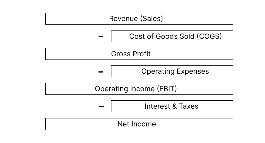
Figure 4 illustrates this progression from total revenue to net income, showing how various costs and expenses are subtracted to arrive at different measure of profit.

Figure 4: A stylized representation of an income statement.

Consider Microsoft’s 2023 income statement in Figure 5, which exemplifies how a leading technology company reports its financial performance:

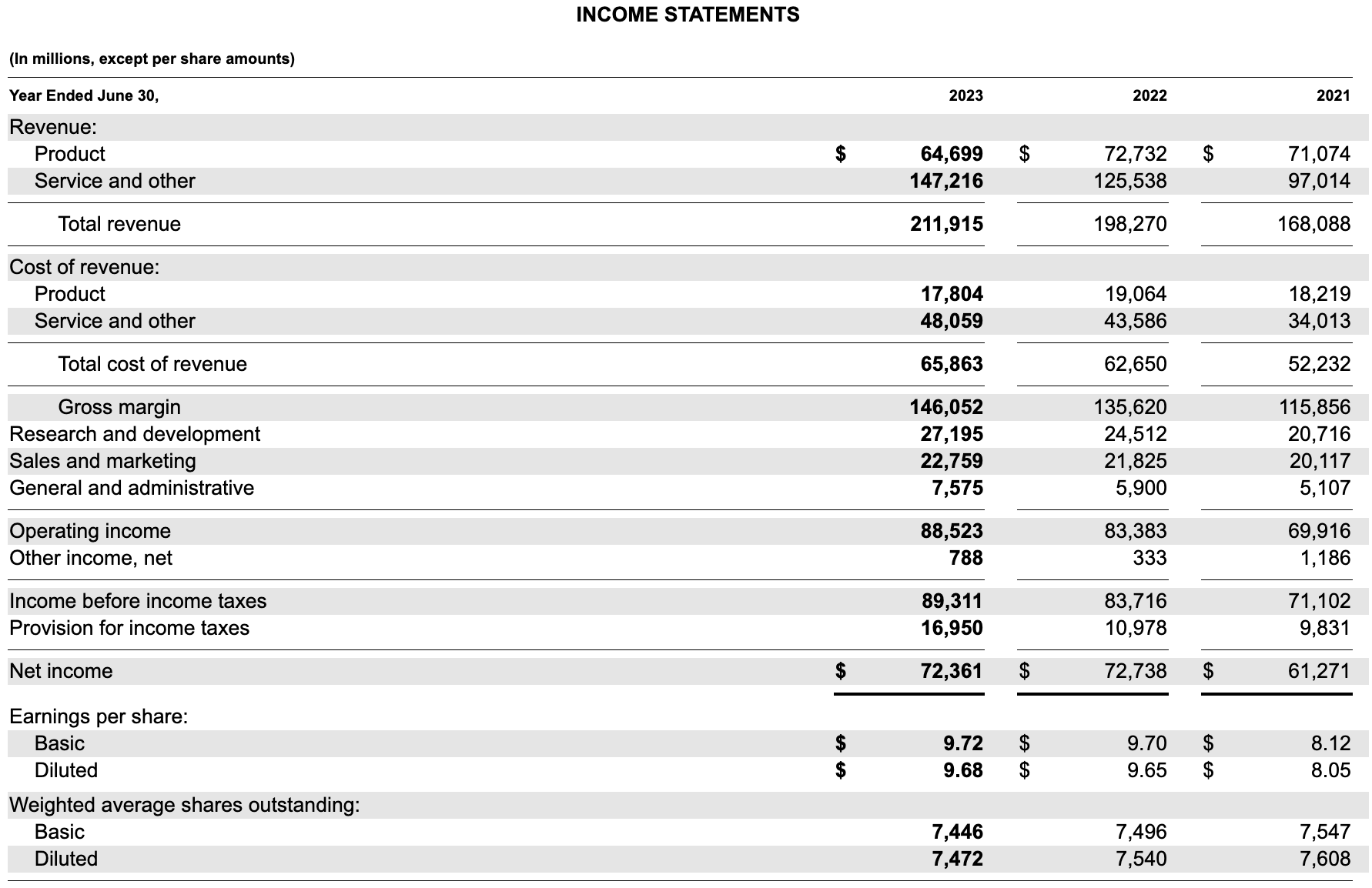
Figure 5: A screenshot of the income statement of Microsoft in 2023.

We can also access this data programmatically using the FMP API:

fmp_get(
  resource = "income-statement",
  symbol = "MSFT",
  params = list(period = "annual", limit = 5)
)

# A tibble: 5 × 39
  date       symbol reported_currency cik        filing_date
  <date>     <chr>  <chr>             <chr>      <date>     
1 2025-06-30 MSFT   USD               0000789019 2025-07-30 
2 2024-06-30 MSFT   USD               0000789019 2024-07-30 
3 2023-06-30 MSFT   USD               0000789019 2023-07-27 
4 2022-06-30 MSFT   USD               0000789019 2022-07-28 
5 2021-06-30 MSFT   USD               0000789019 2021-07-29 
# ℹ 34 more variables: accepted_date <dttm>, fiscal_year <chr>,
#   period <chr>, revenue <dbl>, cost_of_revenue <dbl>,
#   gross_profit <dbl>, research_and_development_expenses <dbl>,
#   general_and_administrative_expenses <dbl>,
#   selling_and_marketing_expenses <dbl>,
#   selling_general_and_administrative_expenses <dbl>,
#   other_expenses <int>, operating_expenses <dbl>, …

fmp_get(
  resource="income-statement",
  symbol="MSFT",
  params={"period": "annual", "limit": 5}
)

shape: (5, 39)

date	symbol	reported_currency	cik	filing_date	accepted_date	fiscal_year	period	revenue	cost_of_revenue	gross_profit	research_and_development_expenses	general_and_administrative_expenses	selling_and_marketing_expenses	selling_general_and_administrative_expenses	other_expenses	operating_expenses	cost_and_expenses	net_interest_income	interest_income	interest_expense	depreciation_and_amortization	ebitda	ebit	non_operating_income_excluding_interest	operating_income	total_other_income_expenses_net	income_before_tax	income_tax_expense	net_income_from_continuing_operations	net_income_from_discontinued_operations	other_adjustments_to_net_income	net_income	net_income_deductions	bottom_line_net_income	eps	eps_diluted	weighted_average_shs_out	weighted_average_shs_out_dil
date	str	str	str	date	datetime[μs]	i32	str	i64	i64	i64	i64	i64	i64	i64	i64	i64	i64	i64	i64	i64	i64	i64	i64	i64	i64	i64	i64	i64	i64	i64	i64	i64	i64	i64	f64	f64	i64	i64
2025-06-30	"MSFT"	"USD"	"0000789019"	2025-07-30	2025-07-30 16:11:40	2025	"FY"	281724000000	87831000000	193893000000	32488000000	7223000000	25654000000	32877000000	0	65365000000	153196000000	262000000	2647000000	2385000000	34153000000	160165000000	126012000000	2516000000	128528000000	-4901000000	123627000000	21795000000	101832000000	0	0	101832000000	0	101832000000	13.7	13.64	7433000000	7465000000
2024-06-30	"MSFT"	"USD"	"0000789019"	2024-07-30	2024-07-30 16:06:22	2024	"FY"	245122000000	74114000000	171008000000	29510000000	7609000000	24456000000	32065000000	0	61575000000	135689000000	222000000	3157000000	2935000000	22287000000	133009000000	110722000000	-1289000000	109433000000	-1646000000	107787000000	19651000000	88136000000	0	0	88136000000	0	88136000000	11.86	11.8	7431000000	7469000000
2023-06-30	"MSFT"	"USD"	"0000789019"	2023-07-27	2023-07-27 16:01:56	2023	"FY"	211915000000	65863000000	146052000000	27195000000	7575000000	22759000000	30334000000	0	57529000000	123392000000	1026000000	2994000000	1968000000	13861000000	105140000000	91279000000	-2756000000	88523000000	788000000	89311000000	16950000000	72361000000	0	0	72361000000	0	72361000000	9.72	9.68	7446000000	7472000000
2022-06-30	"MSFT"	"USD"	"0000789019"	2022-07-28	2022-07-28 16:06:19	2022	"FY"	198270000000	62650000000	135620000000	24512000000	5900000000	21825000000	27725000000	0	52237000000	114887000000	31000000	2094000000	2063000000	14460000000	100239000000	85779000000	-2396000000	83383000000	333000000	83716000000	10978000000	72738000000	0	0	72738000000	0	72738000000	9.7	9.65	7496000000	7540000000
2021-06-30	"MSFT"	"USD"	"0000789019"	2021-07-29	2021-07-29 16:21:55	2021	"FY"	168088000000	52232000000	115856000000	20716000000	5107000000	20117000000	25224000000	0	45940000000	98172000000	-215000000	2131000000	2346000000	11686000000	85134000000	73448000000	-3532000000	69916000000	1186000000	71102000000	9831000000	61271000000	0	0	61271000000	0	61271000000	8.12	8.05	7547000000	7608000000

In later sections, we will use income statement items to calculate important profitability ratios and examine how they compare across companies and industries. The income statement’s focus on performance complements the balance sheet’s position snapshot, providing a more complete picture of a company’s core business operations.

Cash Flow Statements

The cash flow statement complements the balance sheet and income statement by tracking the actual movement of cash through the business. While the income statement shows profitability and the balance sheet shows financial position, the cash flow statement reveals a company’s ability to generate and manage cash - a crucial aspect of every business. The statement is divided into three main categories:

Operating activities: Cash generated from a company’s core business activities (i.e., net income adjusted for non-cash items like depreciation and changes in working capital).
Financing activities: Cash flows related to borrowing, repaying debt, issuing equity, or paying dividends.
Investing activities: Cash spent on or received from long-term investments, such as purchasing or selling property and equipment.

Figure 6 illustrates these three categories of cash flows, which map into changes in the company’s cash balance.

Figure 6: A stylized representation of a cash flow statement.

The statement reconciles accrual-based accounting (used in the income statement) with actual cash movements. This reconciliation is crucial because profitable companies can still face cash shortages, and unprofitable companies might maintain positive cash flow. We complement the brief introduction, by Microsoft’s 2023 cash flow statement in Figure 7.

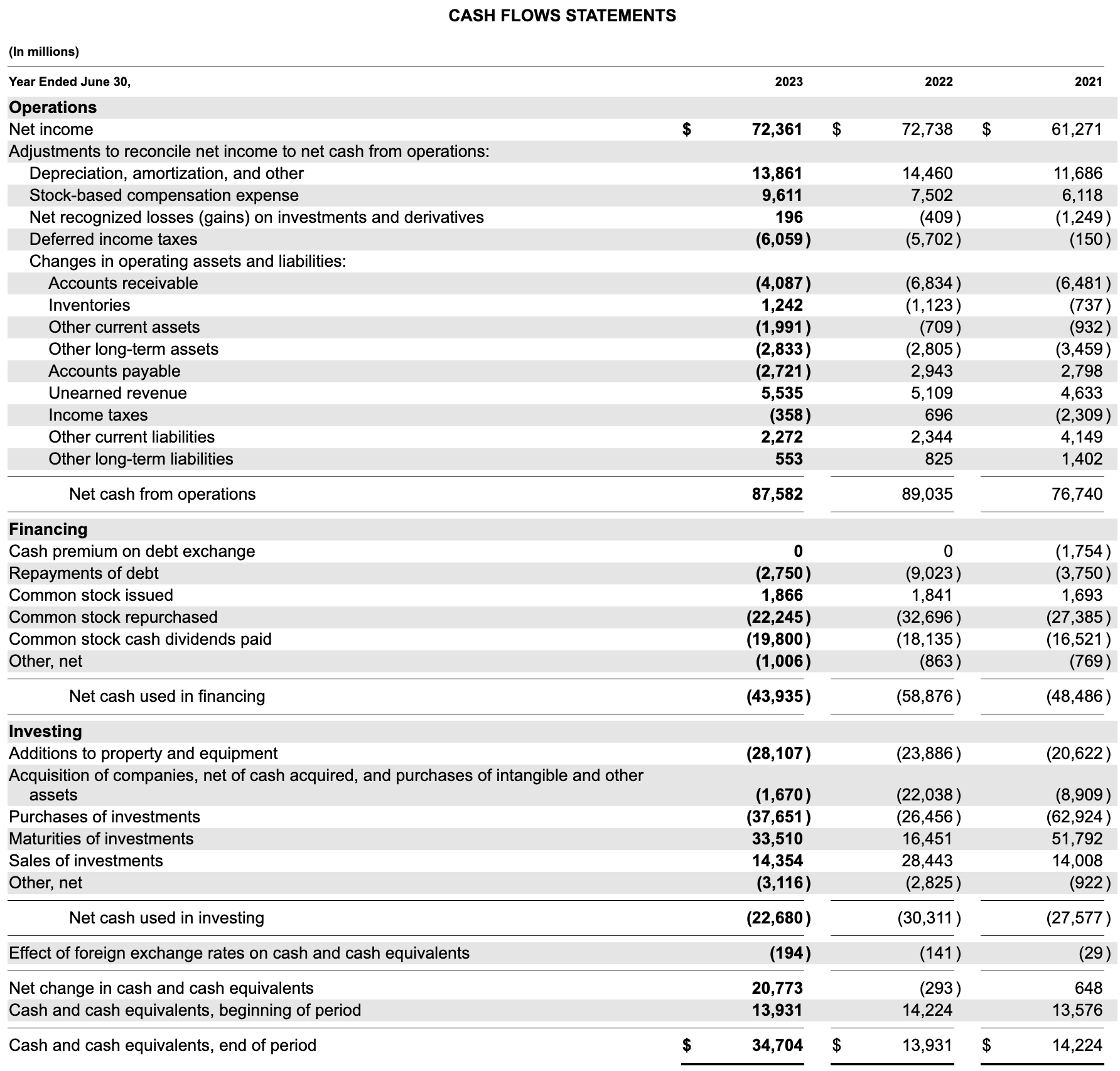
Figure 7: A screenshot of the cash flow statement of Microsoft in 2023.

Of course, we can access this data through the FMP API:

fmp_get(
  resource = "cash-flow-statement",
  symbol = "MSFT",
  params = list(period = "annual", limit = 5)
)

# A tibble: 5 × 47
  date       symbol reported_currency cik        filing_date
  <date>     <chr>  <chr>             <chr>      <date>     
1 2025-06-30 MSFT   USD               0000789019 2025-07-30 
2 2024-06-30 MSFT   USD               0000789019 2024-07-30 
3 2023-06-30 MSFT   USD               0000789019 2023-07-27 
4 2022-06-30 MSFT   USD               0000789019 2022-07-28 
5 2021-06-30 MSFT   USD               0000789019 2021-07-29 
# ℹ 42 more variables: accepted_date <dttm>, fiscal_year <chr>,
#   period <chr>, net_income <dbl>,
#   depreciation_and_amortization <dbl>, deferred_income_tax <dbl>,
#   stock_based_compensation <dbl>, change_in_working_capital <dbl>,
#   accounts_receivables <dbl>, inventory <int>,
#   accounts_payables <dbl>, other_working_capital <dbl>,
#   other_non_cash_items <int>, …

fmp_get(
  resource="cash-flow-statement",
  symbol="MSFT",
  params={"period": "annual", "limit": 5}
)

shape: (5, 47)

date	symbol	reported_currency	cik	filing_date	accepted_date	fiscal_year	period	net_income	depreciation_and_amortization	deferred_income_tax	stock_based_compensation	change_in_working_capital	accounts_receivables	inventory	accounts_payables	other_working_capital	other_non_cash_items	net_cash_provided_by_operating_activities	investments_in_property_plant_and_equipment	acquisitions_net	purchases_of_investments	sales_maturities_of_investments	other_investing_activities	net_cash_provided_by_investing_activities	net_debt_issuance	long_term_net_debt_issuance	short_term_net_debt_issuance	net_stock_issuance	net_common_stock_issuance	common_stock_issuance	common_stock_repurchased	net_preferred_stock_issuance	net_dividends_paid	common_dividends_paid	preferred_dividends_paid	other_financing_activities	net_cash_provided_by_financing_activities	effect_of_forex_changes_on_cash	net_change_in_cash	cash_at_end_of_period	cash_at_beginning_of_period	operating_cash_flow	capital_expenditure	free_cash_flow	income_taxes_paid	interest_paid
date	str	str	str	date	datetime[μs]	i32	str	i64	i64	i64	i64	i64	i64	i64	i64	i64	i64	i64	i64	i64	i64	i64	i64	i64	i64	i64	i64	i64	i64	i64	i64	i64	i64	i64	i64	i64	i64	i64	i64	i64	i64	i64	i64	i64	i64	i64
2025-06-30	"MSFT"	"USD"	"0000789019"	2025-07-30	2025-07-30 16:11:40	2025	"FY"	101832000000	34153000000	-7056000000	11974000000	-5350000000	-10581000000	309000000	569000000	4353000000	609000000	136162000000	-64551000000	-5978000000	-29775000000	25388000000	2317000000	-72599000000	-8962000000	-3216000000	-5746000000	-16364000000	-16364000000	2056000000	-18420000000	0	-24082000000	-24082000000	0	-2291000000	-51699000000	63000000	11927000000	30242000000	18315000000	136162000000	-64551000000	71611000000	0	0
2024-06-30	"MSFT"	"USD"	"0000789019"	2024-07-30	2024-07-30 16:06:22	2024	"FY"	88136000000	22287000000	-4738000000	10734000000	1824000000	-7191000000	1284000000	3545000000	4186000000	305000000	118548000000	-44477000000	-69132000000	-17732000000	35669000000	-1298000000	-96970000000	575000000	-4675000000	5250000000	-15252000000	-15252000000	2002000000	-17254000000	0	-21771000000	-21771000000	0	-1309000000	-37757000000	-210000000	-16389000000	18315000000	34704000000	118548000000	-44477000000	74071000000	0	0
2023-06-30	"MSFT"	"USD"	"0000789019"	2023-07-27	2023-07-27 16:01:56	2023	"FY"	72361000000	13861000000	-6059000000	9611000000	-2388000000	-4087000000	1242000000	-2721000000	3178000000	196000000	87582000000	-28107000000	-1670000000	-37651000000	47864000000	-3116000000	-22680000000	-2750000000	-2750000000	0	-20379000000	-20379000000	1866000000	-22245000000	0	-19800000000	-19800000000	0	-1006000000	-43935000000	-194000000	20773000000	34704000000	13931000000	87582000000	-28107000000	59475000000	0	0
2022-06-30	"MSFT"	"USD"	"0000789019"	2022-07-28	2022-07-28 16:06:19	2022	"FY"	72738000000	14460000000	-5702000000	7502000000	446000000	-6834000000	-1123000000	2943000000	5460000000	-409000000	89035000000	-23886000000	-22038000000	-26456000000	44894000000	-2825000000	-30311000000	-9023000000	-9023000000	0	-30855000000	-30855000000	1841000000	-32696000000	0	-18135000000	-18135000000	0	-863000000	-58876000000	-141000000	-293000000	13931000000	14224000000	89035000000	-23886000000	65149000000	0	0
2021-06-30	"MSFT"	"USD"	"0000789019"	2021-07-29	2021-07-29 16:21:55	2021	"FY"	61271000000	11686000000	-150000000	6118000000	-936000000	-6481000000	-737000000	2798000000	3484000000	-1249000000	76740000000	-20622000000	-8909000000	-62924000000	65800000000	-922000000	-27577000000	-3750000000	-3750000000	0	-25692000000	-25692000000	1693000000	-27385000000	0	-16521000000	-16521000000	0	-2523000000	-48486000000	-29000000	648000000	14224000000	13576000000	76740000000	-20622000000	56118000000	0	0

In subsequent sections, we will use cash flow data to calculate important cash flow ratios that help assess a company’s liquidity, capital allocation efficiency, and overall financial sustainability. The combination of all three financial statements - balance sheet, income statement, and cash flow statement - provides a comprehensive view of a company’s financial health and performance.

Download Financial Statements

We now turn to downloading and processing statements for multiple companies. The next code chunk demonstrates how to retrieve financial data for selected stocks that are supported in the free tier of FMP.

sample <- c(
  "AAPL",
  "MSFT",
  "GOOGL",
  "AMZN",
  "TSLA",
  "NVDA",
  "META",
  "NFLX",
  "DIS",
  "NKE",
  "WMT",
  "KO",
  "JPM",
  "BAC",
  "V",
  "XOM",
  "CVX",
  "JNJ",
  "PFE",
  "INTC",
  "AMD",
  "SBUX",
  "BABA",
  "UBER",
  "CSCO"
)

params <- list(period = "annual", limit = 5)

balance_sheet_statements <- sample |>
  map_df(
    \(x) {
      fmp_get(resource = "balance-sheet-statement", symbol = x, params = params)
    }
  )

income_statements <- sample |>
  map_df(
    \(x) fmp_get(resource = "income-statement", symbol = x, params = params)
  )

cash_flow_statements <- sample |>
  map_df(
    \(x) fmp_get(resource = "cash-flow-statement", symbol = x, params = params)
  )

sample = [
  "AAPL", "MSFT", "GOOGL", "AMZN", "TSLA", "NVDA", "META", "NFLX", "DIS", "NKE",
  "WMT", "KO", "JPM", "BAC", "V", "XOM", "CVX", "JNJ", "PFE", "INTC",
  "AMD", "SBUX", "BABA", "UBER", "CSCO"
]

params = {"period": "annual", "limit": 5}

balance_sheet_statements = pl.concat(
  [fmp_get(
      resource="balance-sheet-statement", symbol=x, params=params
    ) for x in sample]
)

income_statements = pl.concat(
  [fmp_get(
      resource="income-statement", symbol=x, params=params
    ) for x in sample]
)

cash_flow_statements = pl.concat(
  [fmp_get(
      resource="cash-flow-statement", symbol=x, params=params
    ) for x in sample]
)

The resulting data sets provide a foundation for cross-sectional analyses of financial ratios and trends across major U.S. companies. In the following sections, we use these data sets to calculate various financial ratios and analyze patterns in corporate financial performance.

Liquidity Ratios

Liquidity ratios assess a company’s ability to meet its short-term obligations and are typically calculated using balance sheet items. These ratios are particularly important for creditors and investors concerned about a company’s short-term financial health and ability to cover immediate obligations.

The Current Ratio is the most basic measure of liquidity, comparing all current assets to current liabilities:

\[\text{Current Ratio} = \frac{\text{Current Assets}}{\text{Current Liabilities}}\]

A ratio above one indicates that the company has enough current assets to cover its current liabilities, which are due within one year as discussed above.

However, not all current assets are equally liquid, i.e., can be easily sold to meet a company’s obligations. This aspect is reflected in the Quick Ratio:

\[\text{Quick Ratio} = \frac{\text{Current Assets - Inventory}}{\text{Current Liabilities}}\]

The Quick Ratio provides a more stringent measure of liquidity by excluding inventory, which is typically the least liquid current asset. Furthermore, a company without inventory for production or sale will have a difficult operating position. A ratio above one suggests strong short-term solvency without relying on selling off inventory.

The most conservative liquidity measure is the Cash Ratio:

\[\text{Cash Ratio} = \frac{\text{Cash and Cash Equivalents}}{\text{Current Liabilities}}\]

This ratio focuses solely on the most liquid assets - cash and cash equivalents. While a ratio of one indicates robust liquidity, most companies maintain lower cash ratios to avoid holding excessive non-productive assets. After all, all that cash could also be distributed to equity or pay down costly debt.

Next, we calculate these ratios for all stocks, focusing on four major technology companies:

selected_symbols <- c("MSFT", "AAPL", "AMZN", "NVDA")

balance_sheet_statements <- balance_sheet_statements |>
  mutate(
    fiscal_year = as.integer(fiscal_year),
    current_ratio = total_current_assets / total_current_liabilities,
    quick_ratio = (total_current_assets - inventory) /
      total_current_liabilities,
    cash_ratio = cash_and_cash_equivalents / total_current_liabilities,
    label = if_else(symbol %in% selected_symbols, symbol, NA),
  )

selected_symbols = ["MSFT", "AAPL", "AMZN", "NVDA"]

balance_sheet_statements = (balance_sheet_statements
  .with_columns(
    fiscal_year=pl.col("fiscal_year").cast(pl.Int64),
    current_ratio=pl.col("total_current_assets") / pl.col("total_current_liabilities"),
    quick_ratio=(pl.col("total_current_assets") - pl.col("inventory")) / pl.col("total_current_liabilities"),
    cash_ratio=pl.col("cash_and_cash_equivalents") / pl.col("total_current_liabilities"),
    label=pl.when(pl.col("symbol").is_in(selected_symbols)).then(pl.col("symbol")).otherwise(None)
  )
)

Figure 8 compares the three liquidity ratios across Microsoft, Apple, and Amazon for 2023. We call such an analysis a cross-sectional comparison.

balance_sheet_statements |>
  filter(fiscal_year == 2023 & !is.na(label)) |>
  select(symbol, contains("ratio")) |>
  pivot_longer(-symbol) |>
  mutate(name = str_to_title(str_replace_all(name, "_", " "))) |>
  ggplot(aes(x = value, y = name, fill = symbol)) +
  geom_col(position = "dodge") +
  scale_x_continuous(labels = percent) +
  labs(
    x = NULL,
    y = NULL,
    fill = NULL,
    title = "Liquidity ratios for selected stocks for 2023"
  )

Title: Liquidity ratios for selected stocks for 2023. The figure shows a bar chart of liquidity ratios for three companies. — Figure 8: Liquidity ratios are based on financial statements provided through the FMP API.

liquidity_ratios = (balance_sheet_statements
  .filter((pl.col("fiscal_year") == 2023) & pl.col("label").is_not_null())
  .select("symbol", "current_ratio", "quick_ratio", "cash_ratio")
  .unpivot(index=["symbol"], variable_name="name", value_name="value")
  .with_columns(
    name=pl.col("name").str.replace_all("_", " ").str.to_titlecase()
  )
)

liquidity_ratios_figure = (
  ggplot(
    liquidity_ratios,
    aes(y="value", x="name", fill="symbol")
  )
  + geom_col(position="dodge")
  + coord_flip()
  + scale_y_continuous(labels=percent_format())
  + labs(
      x="", y="", fill="",
      title="Liquidity ratios for selected stocks for 2023"
    )
)
liquidity_ratios_figure.show()

While we are not commenting on the ratios in detail here, the liquidity ratios for Microsoft, Apple, and Amazon in 2023 reveal distinct patterns. Generally, higher liquidity ratios signal a more conservative approach by holding larger liquidity buffers in the company.

Leverage Ratios

Leverage ratios assess a company’s capital structure, in particular, its mix between debt and equity. These metrics are crucial for understanding the company’s financial risk and long-term solvency. We examine three key leverage measures.

The debt-to-equity ratio indicates how much a company is financing its operations through debt versus shareholders’ equity:

\[\text{Debt-to-Equity} = \frac{\text{Total Debt}}{\text{Total Equity}}\]

The debt-to-asset ratio shows the percentage of assets financed through debt:

\[\text{Debt-to-Asset} = \frac{\text{Total Debt}}{\text{Total Assets}}\]

Interest coverage measures a company’s ability to meet interest payments:

\[\text{Interest Coverage} = \frac{\text{EBIT}}{\text{Interest Expense}}\]

Let’s calculate these ratios for our sample of companies:

balance_sheet_statements <- balance_sheet_statements |>
  mutate(
    debt_to_equity = total_debt / total_equity,
    debt_to_asset = total_debt / total_assets
  )

income_statements <- income_statements |>
  mutate(
    fiscal_year = as.integer(fiscal_year),
    interest_coverage = operating_income / interest_expense,
    label = if_else(symbol %in% selected_symbols, symbol, NA),
  )

balance_sheet_statements = balance_sheet_statements.with_columns(
  debt_to_equity=pl.col("total_debt") / pl.col("total_equity"),
  debt_to_asset=pl.col("total_debt") / pl.col("total_assets")
)

income_statements = income_statements.with_columns(
  fiscal_year=pl.col("fiscal_year").cast(pl.Int64),
  interest_coverage=pl.col("operating_income") / pl.col("interest_expense"),
  label=pl.when(pl.col("symbol").is_in(selected_symbols)).then(pl.col("symbol")).otherwise(None)
)

Figure 9 tracks the evolution of debt-to-asset ratios for Microsoft, Apple, and Amazon over time:

balance_sheet_statements |>
  filter(symbol %in% selected_symbols) |>
  ggplot(aes(x = fiscal_year, y = debt_to_asset, color = symbol)) +
  geom_line(linewidth = 1) +
  scale_y_continuous(labels = percent) +
  labs(
    x = NULL,
    y = NULL,
    color = NULL,
    title = "Debt-to-asset ratios of selected stocks between 2020 and 2024"
  )

Title: Debt-to-asset ratios of selected stocks between 2020 and 2024. The figure shows a line chart with years on the horizontal axis and debt-to-asset ratios on the vertical axis. — Figure 9: Debt-to-asset ratios are based on financial statements provided through the FMP API.

debt_to_asset = (balance_sheet_statements
  .filter(pl.col("symbol").is_in(selected_symbols))
)

debt_to_asset_figure = (
  ggplot(
    debt_to_asset,
    aes(x="fiscal_year", y="debt_to_asset", color="symbol")
  )
  + geom_line(size=1)
  + scale_y_continuous(labels=percent_format())
  + labs(
      x="", y="", color="",
      title="Debt-to-asset ratios of selected stocks between 2020 and 2024"
    )
)
debt_to_asset_figure.show()

The evolution of debt-to-asset ratios among these major technology companies reveals distinct capital structure strategies and their changes over time. While Apple and Microsoft reduced leverage over time, Amazon has maintained its leverage level.

Figure 10 provides a cross-sectional view of debt-to-asset ratios across our sample in 2023.

balance_sheet_statements |>
  filter(fiscal_year == 2023) |>
  ggplot(
    aes(x = debt_to_asset, y = fct_reorder(symbol, debt_to_asset), fill = label)
  ) +
  geom_col() +
  scale_x_continuous(labels = percent) +  labs(
    x = NULL,
    y = NULL,
    color = NULL,
    title = "Debt-to-asset ratios of selected stocks in 2023"
  ) +
  theme(legend.position = "none")

Title: Debt-to-asset ratios of selected stocks in 2023. The figure shows a bar chart with debt-to-asset ratios on the horizontal and corresponding symbols on the vertical axis. — Figure 10: Debt-to-asset ratios are based on financial statements provided through the FMP API.

debt_to_asset_comparison = (balance_sheet_statements
  .filter(pl.col("fiscal_year") == 2023)
)

symbol_order = (debt_to_asset_comparison
  .sort("debt_to_asset")["symbol"]
  .to_list()
)
debt_to_asset_comparison = debt_to_asset_comparison.with_columns(
  symbol=pl.col("symbol").cast(pl.Enum(symbol_order))
)

debt_to_asset_comparison_figure = (
  ggplot(
    debt_to_asset_comparison,
    aes(y="debt_to_asset", x="symbol", fill="label")
  )
  + geom_col()
  + coord_flip()
  + scale_y_continuous(labels=percent_format())  + labs(
      x="", y="", fill="",
      title="Debt-to-asset ratios of selected stocks in 2023"
    )
  + theme(legend_position="none")
)
debt_to_asset_comparison_figure.show()

Figure 11 reveals the relationship between companies’ debt levels and their ability to service that debt.

income_statements |>
  filter(fiscal_year == 2023) |>
  select(symbol, interest_coverage, fiscal_year) |>
  left_join(
    balance_sheet_statements,
    join_by(symbol, fiscal_year)
  ) |>
  ggplot(aes(x = debt_to_asset, y = interest_coverage, color = label)) +
  geom_point(size = 2) +
  geom_label_repel(aes(label = label), seed = 42, box.padding = 0.75) +
  scale_x_continuous(labels = percent) +
  scale_y_continuous(labels = percent) +  labs(
    x = "Debt-to-Asset",
    y = "Interest Coverage",
    title = "Debt-to-asset ratios and interest coverages for selected stocks"
  ) +
  theme(legend.position = "none")

Title: Debt-to-asset ratios and interest coverages for selected stocks. The figure shows a scatter plot with debt-to-asset on the horizontal and interest coverage on the vertical axis. — Figure 11: Debt-to-asset ratios and interest coverages are based on financial statements provided through the FMP API.

interest_coverage = (income_statements
  .filter(pl.col("fiscal_year") == 2023)
  .select("symbol", "fiscal_year", "interest_coverage")
  .join(balance_sheet_statements, on=["symbol", "fiscal_year"], how="left")
)

interest_coverage_figure = (
  ggplot(
    interest_coverage,
    aes(x="debt_to_asset", y="interest_coverage", color="label")
  )
  + geom_point(size=2)
  + geom_label(aes(label="label"), adjust_text={"arrowprops": {"arrowstyle": "-"}})
  + scale_x_continuous(labels=percent_format())
  + scale_y_continuous(labels=percent_format())  + labs(
      x="Debt-to-Asset", y="Interest Coverage",
      title="Debt-to-asset ratios and interest coverages for selected stocks"
    )
  + theme(legend_position="none")
)
interest_coverage_figure.show()

The scatter plot suggests that companies with higher debt-to-asset ratios tend to have lower interest coverage ratios, though there’s considerable variation in this relation. Quantification of this relation is left as an exercise.

Efficiency Ratios

Efficiency ratios measure how a company utilizes its assets and manages its operations. These metrics help us to understand operational performance and management effectiveness, particularly in how well a company converts its various assets into revenue and profit.

Asset Turnover measures how efficiently a company uses its total assets to generate revenue:

\[\text{Asset Turnover} = \frac{\text{Revenue}}{\text{Total Assets}}\]

A higher ratio indicates more efficient use of assets in generating sales. However, this ratio typically varies significantly across industries - retail companies often have higher turnover ratios due to lower asset requirements, while manufacturing companies might show lower ratios due to substantial fixed asset investments. Such industry-specifics show the importance of cross-sectional comparisons, when making decisions based on data.

Inventory turnover indicates how many times a company’s inventory is sold and replaced over a period:

\[\text{Inventory Turnover} = \frac{\text{COGS}}{\text{Inventory}}\]

Higher inventory turnover suggests more efficient inventory management and working capital utilization. However, extremely high ratios might indicate potential stockouts, while very low ratios could suggest obsolete inventory or overinvestment in working capital.

Receivables turnover measures how effectively a company collects payments from customers:

\[\text{Receivables Turnover} = \frac{\text{Revenue}}{\text{Accounts Receivable}}\] A higher ratio indicates more efficient credit and collection processes, though this must be balanced against the potential impact on sales from overly restrictive credit policies.

Here is how we can calculate these efficiency metrics across our sample of companies:

combined_statements <- balance_sheet_statements |>
  select(
    symbol,
    fiscal_year,
    label,
    current_ratio,
    quick_ratio,
    cash_ratio,
    debt_to_equity,
    debt_to_asset,
    total_assets,
    total_equity
  ) |>
  left_join(
    income_statements |>
      select(
        symbol,
        fiscal_year,
        interest_coverage,
        revenue,
        cost_of_revenue,
        selling_general_and_administrative_expenses,
        interest_expense,
        gross_profit,
        net_income
      ),
    join_by(symbol, fiscal_year)
  ) |>
  left_join(
    cash_flow_statements |>
      mutate(fiscal_year = as.integer(fiscal_year)) |>
      select(symbol, fiscal_year, inventory, accounts_receivables),
    join_by(symbol, fiscal_year)
  )

combined_statements <- combined_statements |>
  mutate(
    asset_turnover = revenue / total_assets,
    inventory_turnover = cost_of_revenue / inventory,
    receivables_turnover = revenue / accounts_receivables
  )

combined_statements = (balance_sheet_statements
  .select(
    "symbol", "fiscal_year", "label", "current_ratio", "quick_ratio",
     "cash_ratio", "debt_to_equity", "debt_to_asset", "total_assets",
     "total_equity"
  )
  .join(
    (income_statements
      .select("symbol", "fiscal_year", "interest_coverage", "revenue",
              "cost_of_revenue", "selling_general_and_administrative_expenses",
              "interest_expense","gross_profit", "net_income")
    ),
    on=["symbol", "fiscal_year"],
    how="left"
  )
  .join(
    (cash_flow_statements
      .with_columns(fiscal_year=pl.col("fiscal_year").cast(pl.Int64))
      .select("symbol", "fiscal_year", "inventory", "accounts_receivables")
    ),
    on=["symbol", "fiscal_year"],
    how="left"
  )
)

combined_statements = (combined_statements
  .with_columns(
    asset_turnover=pl.col("revenue") / pl.col("total_assets"),
    inventory_turnover=pl.col("cost_of_revenue") / pl.col("inventory"),
    receivables_turnover=pl.col("revenue") / pl.col("accounts_receivables")
  )
)

We leave the visualization and interpretation of these figures as an exercise and move on to the last category of financial ratios.

Profitability Ratios

Profitability ratios evaluate a company’s ability to generate earnings relative to its revenue, assets, and equity. These metrics are fundamental to investment analysis as they directly measure a company’s operational efficiency and financial success.

The gross margin measures what percentage of revenue remains after accounting for the direct costs of producing goods or services:

\[\text{Gross Margin} = \frac{\text{Gross Profit}}{\text{Revenue}}\]

A higher gross margin indicates stronger pricing power or more efficient production processes. This metric is particularly useful for comparing companies within the same industry, as it reveals their relative efficiency in core operations before accounting for operating expenses and other costs.

The profit margin reveals what percentage of revenue ultimately becomes net income:

\[\text{Profit Margin} = \frac{\text{Net Income}}{\text{Revenue}}\] This comprehensive profitability measure accounts for all costs, expenses, interest, and taxes. A higher profit margin suggests more effective overall cost management and stronger competitive position, though optimal margins vary significantly across industries.

Return on Equity (ROE) measures how efficiently a company uses shareholders’ investments to generate profits:

\[\text{After-Tax ROE} = \frac{\text{Net Income}}{\text{Total Equity}}\] This metric is particularly important for investors as it directly measures the return on their invested capital (at least in terms of book value of equity). A higher ROE indicates more effective use of shareholders’ equity, though it must be considered alongside leverage ratios since high debt levels can artificially inflate ROE.

The next code chunk calculates these profitability metrics for our sample of companies, allowing us to analyze how different firms convert their revenue into various levels of profit and return on investment.

combined_statements <- combined_statements |>
  mutate(
    gross_margin = gross_profit / revenue,
    profit_margin = net_income / revenue,
    after_tax_roe = net_income / total_equity
  )

combined_statements = combined_statements.with_columns(
  gross_margin=pl.col("gross_profit") / pl.col("revenue"),
  profit_margin=pl.col("net_income") / pl.col("revenue"),
  after_tax_roe=pl.col("net_income") / pl.col("total_equity")
)

Figure 12 shows the patterns in gross margin trends among Microsoft, Apple, and Amazon between 2019 and 2023.

combined_statements |>
  filter(symbol %in% selected_symbols) |>
  ggplot(aes(x = fiscal_year, y = gross_margin, color = symbol)) +
  geom_line() +
  scale_y_continuous(labels = percent) +
  labs(
    x = NULL,
    y = NULL,
    color = NULL,
    title = "Gross margins for selected stocks between 2019 and 2023"
  )

Title: Gross margins for selected stocks between 2019 and 2023. The figure shows a line chart with years on the horizontal axis and gross margins on the vertical axis. — Figure 12: Gross margins are based on financial statements provided through the FMP API.

gross_margins = (combined_statements
  .filter(pl.col("symbol").is_in(selected_symbols))
)

gross_margins_figure = (
  ggplot(
    gross_margins,
    aes(x="fiscal_year", y="gross_margin", color="symbol")
  )
  + geom_line()
  + scale_y_continuous(labels=percent_format())
  + labs(
      x="", y="", color="",
      title="Gross margins for selected stocks between 2019 and 2023"
  )
)
gross_margins_figure.show()

Microsoft maintains the highest margins at 65-70%, reflecting its low-cost software business model, while Apple and Amazon show lower but improving margins from around 40% to 45-47%. This divergence highlights fundamental business model differences.

Figure 13 illustrates the relationship between gross margins and profit margins across our sample of stocks in 2023.

combined_statements |>
  filter(fiscal_year == 2023) |>
  ggplot(aes(x = gross_margin, y = profit_margin, color = label)) +
  geom_point(size = 2) +
  geom_label_repel(aes(label = label), seed = 42, box.padding = 0.75) +
  scale_x_continuous(labels = percent) +
  scale_y_continuous(labels = percent) +  labs(
    x = "Gross margin",
    y = "Profit margin",
    title = "Gross and profit margins for selected stocks in 2023"
  ) +
  theme(legend.position = "none")

Title: Gross and profit margins for selected stocks in 2023. The figure shows a scatter plot with gross margins on the horizontal and profit margins on the vertical axis. — Figure 13: Gross and profit margins are based on financial statements provided through the FMP API.

profit_margins = (combined_statements
  .filter(pl.col("fiscal_year") == 2023)
)

profit_margins_figure = (
  ggplot(
    profit_margins,
    aes(x="gross_margin", y="profit_margin", color="label")
  )
  + geom_point(size=2)
  + geom_label(
      aes(label="label"),
      adjust_text={"arrowprops": {"arrowstyle": "-"}}
    )
  + scale_x_continuous(labels=percent_format())
  + scale_y_continuous(labels=percent_format())  + labs(
      x="Gross margin", y="Profit margin",
      title="Gross and profit margins for selected stocks in 2023"
    )
  + theme(legend_position = "none")
)
profit_margins_figure.show()

Combining Financial Ratios

While individual financial ratios provide specific insights, combining them offers a more comprehensive view of company performance. By examining how companies rank across different ratio categories, we can better understand their overall financial position and identify potential strengths and weaknesses in their operations.

Figure 14 compares Microsoft, Apple, and Amazon’s rankings across four key financial ratio categories among our sample. Rankings closer to 1 indicate better performance within each category.

financial_ratios <- combined_statements |>
  filter(fiscal_year == 2023) |>
  select(
    symbol,
    contains(c(
      "ratio",
      "margin",
      "roe",
      "_to_",
      "turnover",
      "interest_coverage"
    ))
  ) |>
  pivot_longer(cols = -symbol) |>
  mutate(
    type = case_when(
      name %in% c("current_ratio", "quick_ratio", "cash_ratio") ~
        "Liquidity Ratios",
      name %in% c("debt_to_equity", "debt_to_asset", "interest_coverage") ~
        "Leverage Ratios",
      name %in%
        c("asset_turnover", "inventory_turnover", "receivables_turnover") ~
        "Efficiency Ratios",
      name %in% c("gross_margin", "profit_margin", "after_tax_roe") ~
        "Profitability Ratios"
    )
  )

financial_ratios |>
  group_by(type, name) |>
  arrange(desc(value)) |>
  mutate(rank = row_number()) |>
  group_by(symbol, type) |>
  summarize(rank = mean(rank), .groups = "drop") |>
  filter(symbol %in% selected_symbols) |>
  ggplot(aes(x = rank, y = type, color = symbol)) +
  geom_point(shape = 17, size = 4) +  labs(
    x = "Average rank",
    y = NULL,
    color = NULL,
    title = "Average rank among selected stocks"
  ) +
  coord_cartesian(xlim = c(1, 30))

Title: Rank in financial ratio categories for selected stocks. The figure shows a scatter plot with ranks for selected stocks on the horizontal and categories of financial ratios on the vertical axis. — Figure 14: Ranks are based on financial statements provided through the FMP API.

financial_ratios = (combined_statements
  .filter(pl.col("fiscal_year") == 2023)
  .select(
    ["symbol"] + [
      col for col in combined_statements.columns
      if any(x in col for x in ["ratio", "margin", "roe", "_to_", "turnover", "interest_coverage"])
    ]
  )
  .unpivot(index=["symbol"], variable_name="name", value_name="value")
  .with_columns(
    type=pl.when(pl.col("name").is_in(["current_ratio", "quick_ratio", "cash_ratio"]))
      .then(pl.lit("Liquidity Ratios"))
      .when(pl.col("name").is_in(["debt_to_equity", "debt_to_asset", "interest_coverage"]))
      .then(pl.lit("Leverage Ratios"))
      .when(pl.col("name").is_in(["asset_turnover", "inventory_turnover", "receivables_turnover"]))
      .then(pl.lit("Efficiency Ratios"))
      .when(pl.col("name").is_in(["gross_margin", "profit_margin", "after_tax_roe"]))
      .then(pl.lit("Profitability Ratios"))
      .otherwise(pl.lit("Other"))
  )
)

financial_ratios = financial_ratios.with_columns(
  rank=pl.col("value").rank(method="ordinal", descending=True).over("type", "name")
)

final_ranks = (financial_ratios
  .group_by("symbol", "type")
  .agg(rank=pl.col("rank").mean())
  .filter(pl.col("symbol").is_in(selected_symbols))
)

final_ranks_figure = (
  ggplot(
    final_ranks,
    aes(x="rank", y="type", color="symbol")
  )
  + geom_point(shape="^", size=4)  + labs(
      x="Average rank", y="", color="",
      title="Average rank among selected stocks"
  )
  + coord_cartesian(xlim=[1, 30])
)
final_ranks_figure.show()

These combined rankings highlight how different business models and strategies lead to varying financial profiles. This analysis underscores the importance of considering multiple financial metrics together rather than in isolation when evaluating company performance.

Financial Ratios in Asset Pricing

The Fama-French five-factor model aims to explain stock returns by incorporating specific financial metrics ratios. We provide more details in Replicating Fama-French Factors, but here is an intuitive overview:

Size: Calculated as the logarithm of a company’s market capitalization, which is the total market value of its outstanding shares. This factor captures the tendency for smaller firms to outperform larger ones over time.
Book-to-market ratio: Determined by dividing the company’s book equity by its market capitalization. A higher ratio indicates a ‘value’ stock, while a lower ratio suggests a ‘growth’ stock. This metric helps differentiate between undervalued and overvalued companies.
Profitability: Measured as the ratio of operating profit to book equity, where operating profit is calculated as revenue minus cost of goods sold (COGS), selling, general, and administrative expenses (SG&A), and interest expense. This factor assesses a company’s efficiency in generating profits from its equity base.
Investment: Calculated as the percentage change in total assets from the previous period. This factor reflects the company’s growth strategy, indicating whether it is investing aggressively or conservatively.

We can calculate these factors using the FMP API as follows. Since the free tier only supports historical data for the last couple of months, we use the earliest available data that is returned by default:

market_cap <- sample |>
  map_df(
    \(x) {
      fmp_get(
        resource = "historical-market-capitalization",
        x
      )
    }
  ) |>
  filter(date == min(date))

combined_statements_ff <- combined_statements |>
  filter(fiscal_year == 2023) |>
  left_join(market_cap, join_by(symbol)) |>
  left_join(
    balance_sheet_statements |>
      filter(fiscal_year == 2022) |>
      select(symbol, total_assets_lag = total_assets),
    join_by(symbol)
  ) |>
  mutate(
    size = log(market_cap),
    book_to_market = total_equity / market_cap,
    operating_profitability = (revenue -
      cost_of_revenue -
      selling_general_and_administrative_expenses -
      interest_expense) /
      total_equity,
    investment = total_assets / total_assets_lag
  )

market_cap = pl.concat(
  [fmp_get(
      resource="historical-market-capitalization", symbol=x
    ) for x in sample]
)

min_date = market_cap["date"].min()
market_cap = market_cap.filter(pl.col("date") == min_date)

combined_statements_ff = (combined_statements
  .filter(pl.col("fiscal_year") == 2023)
  .join(market_cap, on="symbol", how="left")
  .join(
    (balance_sheet_statements
      .filter(pl.col("fiscal_year") == 2022)
      .select("symbol", "total_assets")
      .rename({"total_assets": "total_assets_lag"})
    ),
    on="symbol", how="left"
  )
  .with_columns(
    size=pl.col("market_cap").log(),
    book_to_market=pl.col("total_equity") / pl.col("market_cap"),
    operating_profitability=(
        (pl.col("revenue") - pl.col("cost_of_revenue") - pl.col("selling_general_and_administrative_expenses") - pl.col("interest_expense"))
        / pl.col("total_equity")
    ),
    investment=pl.col("total_assets") / pl.col("total_assets_lag")
  )
)

Figure 15 shows the ranks of our selected stocks for ratios used in the Fama-French model. The ranks of Microsoft, Apple, and Amazon across Fama-French factors reveal interesting patterns in how these major technology companies align with established asset pricing factors.

combined_statements_ff |>
  select(
    symbol,
    Size = size,
    `Book-to-Market` = book_to_market,
    `Profitability` = operating_profitability,
    Investment = investment
  ) |>
  pivot_longer(-symbol) |>
  group_by(name) |>
  arrange(desc(value)) |>
  mutate(rank = row_number()) |>
  ungroup() |>
  filter(symbol %in% selected_symbols) |>
  ggplot(aes(x = rank, y = name, color = symbol)) +
  geom_point(shape = 17, size = 4) +  labs(
    x = "Rank",
    y = NULL,
    color = NULL,
    title = "Rank in Fama-French variables for selected stocks"
  ) +
  coord_cartesian(xlim = c(1, 30))

Title: Rank in Fama-French variables for selected stocks. The figure shows a scatter plot with ranks for selected stocks on the horizontal and Fama-French variables on the vertical axis. — Figure 15: Ranks are based on financial statements and historical market capitalization provided through the FMP API.

factors_ranks = (combined_statements_ff
  .select("symbol", "size", "book_to_market", "operating_profitability", "investment")
  .rename({
    "size": "Size",
    "book_to_market": "Book-to-Market",
    "operating_profitability": "Profitability",
    "investment": "Investment"
  })
  .unpivot(index=["symbol"], variable_name="name", value_name="value")
  .with_columns(
    rank=pl.col("value").rank(method="ordinal", descending=True).over("name")
  )
  .filter(pl.col("symbol").is_in(selected_symbols))
)

factors_ranks_figure = (
  ggplot(
    factors_ranks,
    aes(x="rank", y="name", color="symbol")
  )
  + geom_point(shape="^", size=4)  + labs(
      x="Rank", y="", color="",
      title="Rank in Fama-French variables for selected stocks"
  )
  + coord_cartesian(xlim=[1, 30])
)
factors_ranks_figure.show()

As expected, all three tech giants rank among the largest firms by size. Apple shows the highest profitability among the three tech giants according to the new measure, while Microsoft ranks only in the middle. In terms of investment, however, Apple ranks in the lower third of the distribution. All three stocks exhibit relatively low book-to-market ratios—typical of growth stocks—but only when compared to other stocks in our sample.

Key Takeaways

Financial statements offer structured insights into a company’s financial health by summarizing its assets, liabilities, equity, revenues, expenses, and cash flows.
Liquidity ratios, such as the current, quick, and cash ratios, help assess a company’s ability to meet short-term obligations using different levels of liquid assets.
Leverage ratios, including debt-to-equity and debt-to-asset, measure how a company finances its operations and indicate long-term financial risk and capital structure.
Profitability ratios, such as gross margin, profit margin, and return on equity, show how effectively a company turns revenues and investments into earnings.
Efficiency ratios, including asset turnover and inventory turnover, highlight how well a company manages its assets and operations to generate sales.
Financial ratios also serve as key inputs in asset pricing models, such as the Fama-French five-factor model, linking corporate fundamentals to expected stock returns.

Exercises

Download the financial statements for Netflix (NFLX) using the FMP API. Calculate its current ratio, quick ratio, and cash ratio for the past three years. Create a line plot showing how these liquidity ratios have evolved over time. How do Netflix’s liquidity ratios compare to those of the technology companies discussed in this chapter?
Select three companies from different industries. Calculate their debt-to-equity ratios, debt-to-asset ratios, and interest coverage ratios. Create a visualization comparing these leverage metrics across the companies. Write a brief analysis explaining how and why leverage patterns differ across industries.
For all stocks in the sample above, calculate asset turnover, inventory turnover, and receivables turnover. Create a scatter plot showing the relationship between asset turnover and profitability. Identify any outliers and explain potential reasons for their unusual performance. Which industries tend to show higher efficiency ratios? Why might this be the case?
Revisit the scatter plot of debt-to-asset ratios and interest coverages by adding a regression line and quantifying the relationship between the two variables. How can you describe their relationship?