| Variable name | Variable type | Data type |
|---|---|---|
| Quoted bid-ask spread | Liquidity | Quote tick data |
| Quoted depth | Liquidity | Quote tick data |
| Effective bid-ask spread | Liquidity | Quote and trade tick data |
| Trade volume | Volume | Trade tick data |
| Price impact | Liquidity | Quote and trade tick data |
| Realized spread | Liquidity | Quote and trade tick data |
| Return autocorrelation | Efficiency | Equispaced quote data |
| Realized volatility | Volatility | Equispaced quote data |
| Variance ratio | Efficiency | Equispaced quote data |
Anyone active in market microstructure research knows that the devil is in the details. When clocks tick in microseconds and prices move in cents, a brief delay or a small fee discount can make a huge difference for traders. In fact, they can even be the business model of an exchange. But as much as such institutional detail is fascinating, the empirical implementation of even the most conventional microstructure concepts can be frustrating. Referring to the interest of brevity, many journal articles often defer the implementation details to an appendix, and even there they tend to be vague or incomplete. With the additional challenge of vast data sets, new entrants into this field face a steep challenge.
We provide a beginner’s guide to market quality measurement in high-frequency data, aiming to lower the barriers to entry into empirical market microstructure. We discuss economic considerations and show step-by-step how to code the most common measures of market liquidity and market efficiency. Because virtually all securities now trade at multiple venues, we also emphasize how market quality can account for market fragmentation.
Is this guide really needed? Well, a recent paper by Menkveld et al., (2023)1 shows in full clarity that even small variations in methodology can lead to large differences in market quality measures. The authors assigned the same set of market microstructure hypotheses and the same data to 164 research teams. They found that the variation in results across teams, the non-standard error, was of a magnitude similar to the standard error. Many teams included seasoned professors, but past publication performance and seniority did not reduce the non-standard error.
Another question is if the cumbersome high-frequency data analysis is really worth the effort? After all, there are numerous liquidity proxies based on daily data. The answer depends on the research question. First, low-frequency proxies are designed for low-frequency applications. For example, Amihud’s (2002)2 popular proxy was originally proposed to be measured as an annual average. Most microstructure applications require liquidity measures at higher frequencies than that. Furthermore, recent evidence by Jahan-Parvar and Zikes (2023)3 show that many low-frequency proxies capture volatility rather than liquidity.
If we convinced you to take on the high-frequency data, here’s what we offer. Table 1 lists the market quality measures that we cover, as well as their underlying data type. For some measures, we include several versions and discuss the differences between them. We organize the text by the data type, as we think that is a natural work flow. We start with liquidity measures based on tick-by-tick quote data, followed by measures based on both trade and quote data. Finally, we look into a set of measures of efficiency and volatility that require equispaced quote data.
Our focus is on the practice of empirical market microstructure. As such, we often motivate the coding choices with economic concepts. Other than that, however, readers interested in the economics underlying each metric are referred to introductory texts such as Campbell, Lo and MacKinlay (1997)4, Foucault, Pagano & Röell (2013)5 and Hasbrouck (2007)6.
Programming
The coding here is in R.
The choice of language is of course a matter of taste. When deciding on the tools to use, what is important to consider is that the data files in this field are often huge. How can we process them without crashing our laptops? The example data used in this guide are tiny, but we wrote the code to be efficient when the number of observations per day go from thousands to millions.7
Even within the world of R, there are of course different packages available to pursue the same goal. We primarily rely on data.table, which is a very fast package for working with the high dimensional data that characterizes microstructure. The speed benefits show when reading and sorting data, and really shine when applying functions to several groups.8
The basic data.table syntax takes the form DT[i, j, by], where i and j can be used to subset or reorder rows and columns much in the same way as in a data.frame. In addition, j can be used to define new variables either for the full data set or group-wise as specified in the by argument. We will give examples and introduce more data.table syntax as we go along. A more complete intro to the package can be found here.
For readers following the Tidy Finance project of Scheuch et al. (2023)9, the data.table syntax can become a friction. For this reason, this guide comes in two flavors. As an alternative to data.table, we also show how to achieve essentially the same virtues in speed, but using the tidyverse syntax. The latter is based on dtplyr, which provides a data.table backend for the familiar dplyr package. Since the example data in this post is fairly small with around 250k rows, there are hardly any performance benefits of data.table over other packages. In practice, however, one works with billions of rows and the benefits of data.table manifest quickly.
Data
We use one week of quote and trade data for one stock (PRU, Prudential Financial Inc.). There is nothing special about that stock – it is chosen to be representative of large-cap stocks in general. As is typical these days, PRU is traded at several exchanges as well as off-exchange. In addition to the listing venue (London Stock Exchange, LSE), the data includes trades and quotes from the competing venue Turquoise (TQE), as well as some dark pool trades.
The data is loaded automatically in the scripts provided. It can also be downloaded manually here.
The data are extracted from the Tick History database, available from the London Stock Exchange Group (LSEG). We are grateful to LSEG for giving us permission to post the example data in the public domain. It is to be used for educational purposes only. The data set is incomplete in that it excludes quotes and trades from numerous venues where the same stock is traded. For the illustrative purpose here, however, two exchanges suffice.
Quote-based liquidity
The most well-known liquidity measure is probably the quoted bid-ask spread. It measures the cost of a hypothetical roundtrip trade, where an investor buys one share only to immediately sell it again. Even though such a trade is not economically sensible, the quoted spread offers a liquidity snapshot that is accessible at any time when the market is open. All that is required is the best bid and ask prices, , the highest bid price and the lowest ask price. Such data typically also come with the number of shares that is available at each price, allowing for a similar snapshot of market depth. That is, the maximum size that can be traded at the best price.
Quotes are expressions of interests to buy or sell securities, observable before a trading decision is made. The quotes that we access in the examples below come from limit order book (LOB) markets, but they may just as well be posted by dealers in request for quote systems, or shouted by specialists in a trading pit.
Quote data inspection and preparation
Let’s dive into it. After loading the required packages, the following code shows how to import and preview the data. We get an overview of the data by simply typing the name of the data frame in the console. It automatically abbreviates the content to show only a subset of the data.
The data can be downloaded directly from within R.
quotes_url <- "http://tinyurl.com/pruquotes"To load the data we use the function ‘fread’ which is similar to read.csv, but much faster.
# Install and load the `data.table` package
# install.packages("data.table")
library(data.table)

# Load the view the quote data
quotes <- fread(quotes_url)
The raw data looks as follows.
quotes #RIC Domain Date-Time GMT Offset Type Bid Price
1: PRU.L Market Price 2021-06-07 04:00:03 1 Quote 1450.0
2: PRU.L Market Price 2021-06-07 06:50:00 1 Quote 1450.0
3: PRU.L Market Price 2021-06-07 06:50:00 1 Quote 1450.0
4: PRU.L Market Price 2021-06-07 06:50:00 1 Quote 1450.0
5: PRU.L Market Price 2021-06-07 06:50:00 1 Quote 1450.0
---
263969: PRUl.TQ Market Price 2021-06-11 15:29:59 1 Quote 1488.5
263970: PRUl.TQ Market Price 2021-06-11 15:29:59 1 Quote 1488.5
263971: PRUl.TQ Market Price 2021-06-11 15:29:59 1 Quote NA
263972: PRUl.TQ Market Price 2021-06-11 15:30:00 1 Quote NA
263973: PRUl.TQ Market Price 2021-06-11 15:30:00 1 Quote NA
Bid Size Ask Price Ask Size Exch Time
1: 300 1550.0 700 04:00:02.983920000
2: 1028 1550.0 700 06:50:00.016246000
3: 1028 1510.5 1000 06:50:00.251314000
4: 1028 1504.5 1000 06:50:00.402760000
5: 1028 1504.5 1009 06:50:00.547739000
---
263969: 476 1496.0 472 15:29:59.623000000
263970: 476 1600.0 425 15:29:59.798000000
263971: NA 1600.0 425 15:29:59.833000000
263972: NA 1600.0 325 15:30:00.104000000
263973: NA NA NA 15:30:00.104000000# install.packages("data.table")
# install.packages("dtplyr")
# install.packages("tidyverse")
library(data.table)
library(dtplyr)
library(tidyverse)We read the data as a tibble using the (very fast) function read_csv. The call lazy_dt converts the tibble to a lazy data.table object. Lazy means that all following commands are not executed immediately but translated to data.table syntax first and then executed at a final stage. As a result, there should be almost no difference in execution time of the code in tidyverse syntax versus the data.table implementation.
tv_quotes <- read_csv(quotes_url, col_types = list(`Exch Time` = col_character()))

tv_quotes <- lazy_dt(tv_quotes)
The raw data looks as follows.
tv_quotesSource: local data table [263,973 x 10]
Call: `_DT1`
`#RIC` Domain `Date-Time` `GMT Offset` Type `Bid Price` `Bid Size`
<chr> <chr> <dttm> <dbl> <chr> <dbl> <dbl>
1 PRU.L Market P… 2021-06-07 04:00:03 1 Quote 1450 300
2 PRU.L Market P… 2021-06-07 06:50:00 1 Quote 1450 1028
3 PRU.L Market P… 2021-06-07 06:50:00 1 Quote 1450 1028
4 PRU.L Market P… 2021-06-07 06:50:00 1 Quote 1450 1028
5 PRU.L Market P… 2021-06-07 06:50:00 1 Quote 1450 1028
6 PRU.L Market P… 2021-06-07 06:50:05 1 Quote 1450 1035
# ℹ 263,967 more rows
# ℹ 3 more variables: `Ask Price` <dbl>, `Ask Size` <dbl>, `Exch Time` <chr>
# Use as.data.table()/as.data.frame()/as_tibble() to access resultsNote that we use the suffix tv_ for every object generated using tidyverse syntax. This way you can execute the entire code of this guide without overwriting data.table objects with the dtplyr equivalent and vice versa.
The data contain four variables that describe the state of the order book (Bid Price, Bid Size, Ask Price, and Ask Size). The LOB holds orders at numerous different prices, but we only see the best price level on each side. This is sufficient for most quote-based market quality measures. We also get three variables conveying time stamps and time zone information (Date-Time, GMT Offset, and Exch time; discussed in detail below), and three character variables (#RIC, Domain, and Type).
Before processing the data, we rename the variables. Names containing spaces, hashes, and dashes may make sense for data vendors, but they are impractical to work with in R. Furthermore, for the order book variables, we prefer to use the term depth to refer to the number of shares quoted, reserving the term size to the number of shares changing hands in a trade.
The command setnames replaces the existing variables with our desired column names.
raw_quote_variables <- c("#RIC", "Date-Time", "GMT Offset", "Domain", "Exch Time",
                         "Type", "Bid Price", "Bid Size", "Ask Price", "Ask Size")

new_quote_variables <- c("ticker", "date_time", "gmt_offset", "domain", "exchange_time",
                         "type", "bid_price", "bid_depth", "ask_price", "ask_depth")

setnames(quotes, raw_quote_variables, new_quote_variables)
tv_quotes <- tv_quotes|>
rename(ticker = `#RIC`,
domain = Domain,
date_time = `Date-Time`,
gmt_offset = `GMT Offset`,
type = Type,
bid_price = `Bid Price`,
bid_depth = `Bid Size`,
ask_price = `Ask Price`,
ask_depth = `Ask Size`,
exchange_time = `Exch Time`
) |>
lazy_dt()From the output above, the character columns might look like they are the same for all rows, hence occupying more memory than necessary. The data.table::table() or dtplyr::count() functions are great to gauge the variation in categorical variables. In this case, it shows us that there is variation in the ticker variable. The two tickers are for the same stock, PRU, traded at two different exchanges, LSE and TQE. The former is more active, with 165,261 quote updates.
The other two character variables, domain and type, are indeed constants. We delete them to save memory.
# Output a table of sample tickers and values of `domain` and `type`
table(quotes$ticker, quotes$type, quotes$domain)
, , = Market Price
Quote
PRU.L 165261
PRUl.TQ 98712# Delete variables
quotes[, c("domain", "type") := NULL]tv_quotes |>
count(ticker, type, domain)Source: local data table [2 x 4]
Call: `_DT2`[, .(n = .N), keyby = .(ticker, type, domain)]
ticker type domain n
<chr> <chr> <chr> <int>
1 PRU.L Quote Market Price 165261
2 PRUl.TQ Quote Market Price 98712
# Use as.data.table()/as.data.frame()/as_tibble() to access resultstv_quotes <- tv_quotes |>
select(-type, -domain)Dates
In the raw data, dates and times are embedded in the same variable, date_time, but for us it is useful to have them in separate variables. Accordingly, we now define the variable date.
Note here that the operator := is used to define a new variable (date) within an existing data.table, such as quotes in this example. Within a data.table, it suffices to refer to the variable name, date_time, when defining the new variable. This is different to a data.frame, for which we would have to write quotes$date_time.
# Obtain dates
quotes[, date := as.Date(date_time)]

# Output a table of sample dates and tickers
table(quotes$ticker, quotes$date)
          2021-06-07 2021-06-08 2021-06-09 2021-06-10 2021-06-11
  PRU.L        27415      38836      30962      39639      28409
  PRUl.TQ      16424      26040      18207      21170      16871
tv_quotes <- tv_quotes |>
mutate(date = as.Date(date_time)) |>
lazy_dt()
tv_quotes |>
count(ticker, date) |>
pivot_wider(names_from = ticker,
values_from = n)Source: local data table [5 x 3]
Call: dcast(`_DT3`[, .(n = .N), keyby = .(ticker, date)], formula = date ~
ticker, value.var = "n")
date PRU.L PRUl.TQ
<date> <int> <int>
1 2021-06-07 27415 16424
2 2021-06-08 38836 26040
3 2021-06-09 30962 18207
4 2021-06-10 39639 21170
5 2021-06-11 28409 16871
# Use as.data.table()/as.data.frame()/as_tibble() to access resultsThe table output shows that there are five trading days in the sample. The number of quote observations per stock-date varies between roughly 16,000 and 40,000. The tendency that LSE has more quotes than TQE is consistent across trading days.
Timestamps
The accuracy of timestamps is important in microstructure data. Timestamps are often matched between quote and trade data (that are not necessarily generated in the same systems), or between data from exchanges in different locations. It is thus essential to be aware of latencies that may arise due to geography or hardware, for example.
We have two timestamps for each observation. The exchange_time variable is assigned by the exchange at the time an event is recorded in the exchange matching engine. The date_time variable is the timestamp assigned on receipt at the data vendor, which is by definition later than the exchange_time. Exchanges that are located at different distances from the vendor are likely to have different reporting delays. It is then up to the researcher to determine which timestamp to rely on, and the choice may depend on the research question. In our setting, as we measure liquidity across venues, it is important that the time stamps across venues are comparable. Based on that each exchanges has strong incentives to assign accurate time stamps (to cater for low-latency participants), we choose to work with the exchange_time variable.
For US equity markets, the timestamp may reflect the matching engine time, the time when the national best bid and offer updates, or the participant timestamp. For discussions about which of these to use, see Bartlett & McCrary (2019)10, Holden, Pierson & Wu (2023)11, and Schwenk-Nebbe (2021)12.
When working with timestamps in microstructure applications, it is useful to convert them into a numeric format. Dedicated time formats (e.g., xts) are imprecise when it comes to sub-second units (see here and here). We thus convert the timestamps to the number of seconds elapsed since midnight. For example, 8:30 am becomes 8.5 x 3,600 = 30,600, because there are 3,600 seconds per hour.
The code below converts exchange_time to numeric and adjusts it for daylight saving using the gmt_offset variable (which is measured in hours). Note the use of curly brackets {...} in the definition of the time variable, which allows us to temporarily define the variable time_elements within the call. Once the operation is complete, the temporary variable is automatically deleted. The variable that is retained should always be returned as a list, hence list(time).
# Convert time stamps to numeric format, expressed in seconds past midnight
# The function `strsplit` splits a character string at the point defined by `split`
# `do.call` is a way to call a function, which in this case calls `rbind` to convert a
# list of vectors to a matrix, where each vector forms one row
quotes[, time := {
    time_elements = strsplit(exchange_time, split = ":")
    time_elements = do.call(rbind, time_elements)
    time = as.numeric(time_elements[, 1]) * 3600 +
           as.numeric(time_elements[, 2]) * 60 +
           as.numeric(time_elements[, 3]) +
           gmt_offset * 3600
    list(time)}]
Having made sure that dates and times are in the desired format, we can save space by dropping the raw time and date variables.
quotes[, c("date_time", "exchange_time", "gmt_offset") := NULL]tv_quotes <- tv_quotes |>
separate(exchange_time,
into = c("hour", "minute", "second"),
sep=":",
convert = TRUE) |>
mutate(time = hour * 3600 + minute * 60 + second + gmt_offset * 3600)Having made sure that dates and times are in the desired format, we can save space by dropping the raw time and date variables.
tv_quotes <- tv_quotes|>
  select(-c("date_time", "gmt_offset","hour","minute","second"))
Prices and depths
An important feature of LOB quotes is that they remain valid until cancelled, executed or modified. Whenever there is a change to the prevailing quotes, a new quote observation is added to the data. It is irrelevant if the latest quote is from the previous millisecond or from the previous minute – it remains valid until updated. It is thus economically meaningful to forward-fill quotes that prevailed in the previous period. Trades, in contrast, are agreed upon at a fixed point in time and do not convey any information about future prices or sizes. They should not be forward-filled, see Hagströmer and Menkveld (2023)13.
When forward-filling quote data, it is important to restrict the procedure to the same date, stock and trading venue. For example, quotes should never be forward-filled from one day to the next, and not from one venue to another. This is ensured with the by argument (in data.table) or the group_by function (in tidyverse), which specifies that the operation is to be done within each combination of tickers and dates.
We use the nafill function to forward-fill, with the option type = "locf" (last observation carried forward) specifying the type of filling. The .SD inside the lapply command tells data.table to repeat the same operation for the set of variables specified by the option .SDcols.
In summary, whereas the .SD applies the same function across a set of variables (columns), the by applies it across categories of observations (rows). The same outcome could be achieved with for loops, but in R, that would be much slower. We discuss that further below.
Note here how the := notation can be used to define multiple variables, using a vector of variable names on the left-hand-side and a function (in this case lapply) that returns a list of variables on the right-hand-side. Note also that when referring to multiple variable names within the data.table, they are specified as a character vector.
# Forward-fill quoted prices and depths
lob_variables <- c("bid_price", "bid_depth", "ask_price", "ask_depth")

quotes[,
  (lob_variables) := lapply(.SD, nafill, type = "locf"),    .SDcols = (lob_variables),
  by = c("ticker", "date")]
tv_quotes <- tv_quotes |>
group_by(ticker, date) |>
fill(matches("bid|ask")) |>
ungroup()When measuring market quality in continuous trading, it is common to filter out periods that may be influenced by call auctions. The LSE opens for trading with a call auction at 08:00 am, local time, and closes with another call at 4:30 pm. There is also an intraday call auction at noon, 12:00 pm. To avoid the impact of the auctions, we exclude quotes before 8:01 am and after 4:29 pm. We do not exclude quotes recorded around the intraday call auction, but set them as missing (NA). If they were instead deleted, it would give the false impression that the last observation before the excluded quotes was still valid.
When entering the opening hours, remember to state them for the same time zone as recorded in the data. In our case, the gmt_offset adjustment above makes sure that the data is stated in local (London) time.
open_time <- 8 * 3600
close_time <- 16.5 * 3600
intraday_auction_time <- 12 * 3600
First, we exclude quotes around the opening and closing of continuous trading. Next, we set quotes around the intraday auction to missing.
quotes <- quotes[time > (open_time + 60) & time < (close_time - 60)]quotes[time > (intraday_auction_time - 60) & time < (intraday_auction_time + 3 * 60),
(lob_variables)] <- NAtv_quotes <- tv_quotes |>
filter(time > hms::as_hms("08:01:00"),
time < hms::as_hms("16:29:00"))
tv_quotes <- tv_quotes |>
mutate(across(matches("bid|ask"),
~if_else(time > hms::as_hms("11:59:00") &
time < hms::as_hms("12:03:00"), NA_real_, .))) |>
lazy_dt()Screening
Before turning to the market quality measurement, it is a good habit to check that the quote observations make economic sense. One way to do that is to study the variation in the bid-ask spread. The nominal bid-ask spread is defined as the difference between the ask price, \(P^A\), and the bid price, \(P^B\), \(\text{quoted}\_\text{spread}^{nom}= P^A - P^B\). A histogram offers a quick overview of the variation (a line plot of the prices is also useful, see Section 2.1).
In the output below, note that the x-axis is in units of pence (0.01 British Pounds, GBP). All quoted prices in this example data follow that convention. Note also that the bid-ask spread is strictly positive, as it should be whenever the market is open. The TQE occasionally has wider spreads than the LSE, but there are no extraordinarily large spreads. The maximum spread, GBP 0.11, corresponds to around 0.7% of the stock price.
Also, it is clear from the histogram that the tick size, the minimum price increment that is allowed when quoting prices, is 0.5 pence (that is, GBP 0.005). Most spreads are quoted at one or two ticks.
We use the package ggplot2 to plot an histogram of the nominal quoted bid-ask spreads.
library(ggplot2)
ggplot(quotes,
       aes(x = ask_price - bid_price, fill = ticker)) +
  geom_histogram(bins = 100) +
  labs(title = "Histogram of nominal bid-ask spread",
       x = "Nominal bid-ask spread (pence)",
       y = "Count",
       fill = NULL) +
  scale_x_continuous(breaks = 1:12)
Warning: Removed 1576 rows containing non-finite values (`stat_bin()`).
tv_quotes |>
  as_tibble() |>
  ggplot(aes(x = ask_price - bid_price, fill = ticker)) +
  geom_histogram(bins = 100) +
  labs(title = "Histogram of nominal bid-ask spread",
       x = "Nominal bid-ask spread (pence)",
       y = "Count",
       fill = NULL) +
  scale_x_continuous(breaks = 1:12)
Warning: Removed 1576 rows containing non-finite values (`stat_bin()`).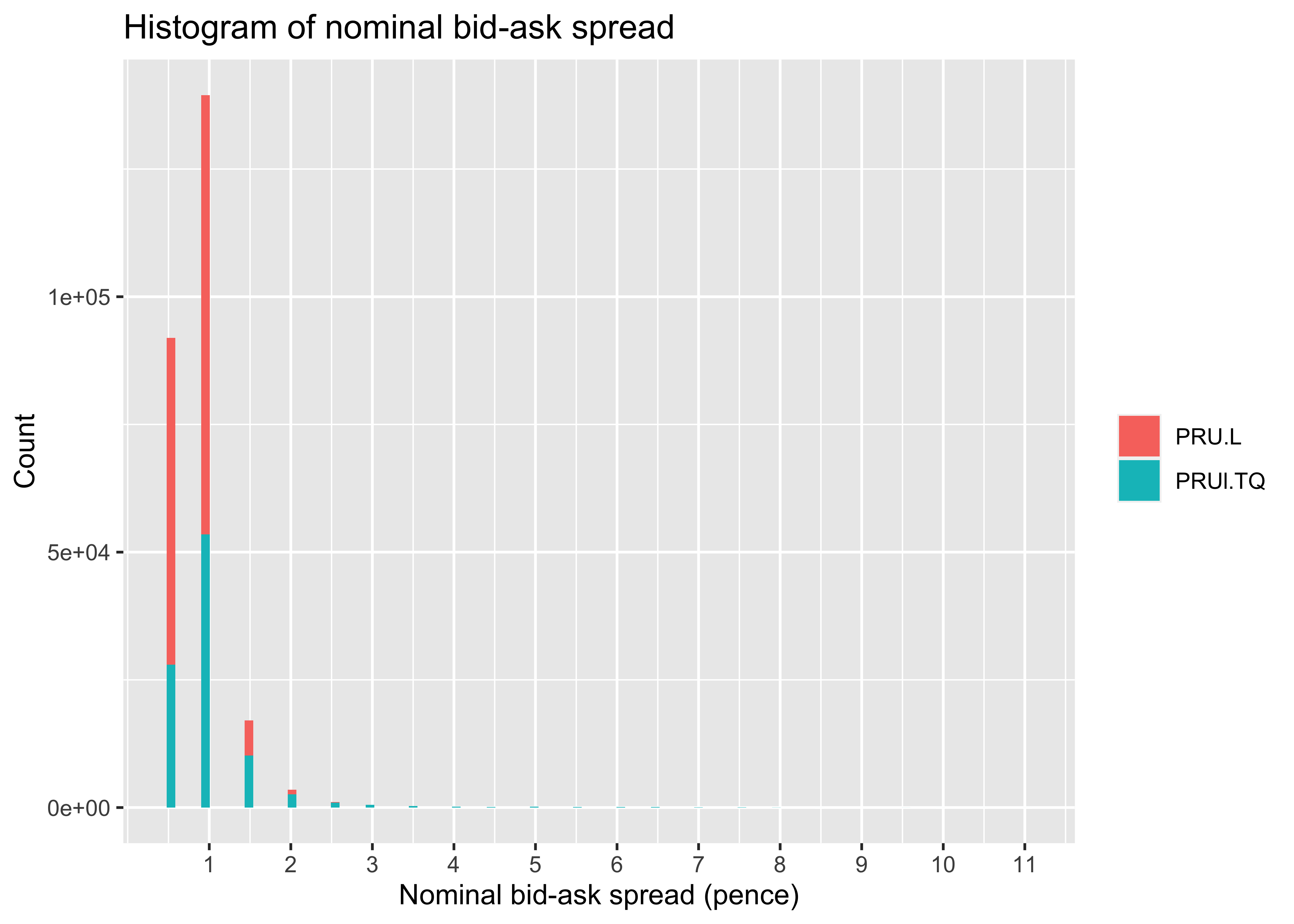
R produces a warning when plotting the nominal bid-ask spread. It mentions 1,576 rows containing “non-finite values”. The non-finite values refer either NA, Inf (infinite) or -Inf (negative infinite). In the timestamp section, we imposed NA for LOB variables during midday auction. To see if those are the cause of the warning, let’s create a histogram of the time stamps of the missing values.
Indeed, all missing values are around ~43,150 and ~43,350 seconds of the trading day which is the time of the midday auction (noon is \(12\times3,600=43,200\) seconds past midnight). Accounting for missing spreads by plotting the histogram without NA removes the warning.
# Plot a histogram of missing quoted spreads
ggplot(quotes[is.na(ask_price - bid_price)],
       aes(x = time, fill = ticker)) +
  geom_histogram(bins = 100) +
  labs(title = "Histogram of missing spreads",
       x = "Time of Day (seconds past midnight)",
       y = "Count")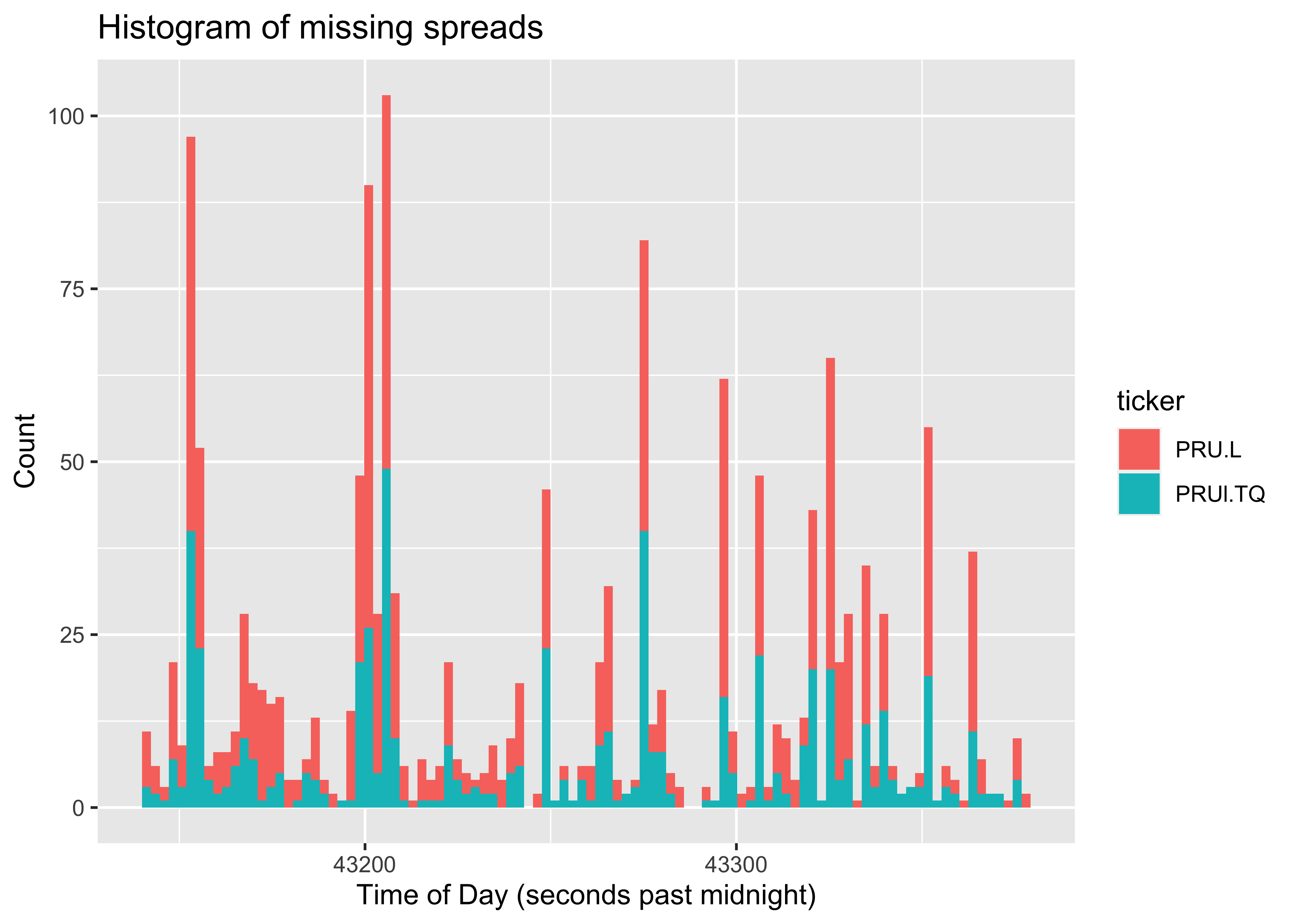
tv_quotes |>
  filter(is.na(ask_price) | is.na(bid_price)) |>
  mutate(time = hms::hms(time)) |>
  as_tibble() |>
  ggplot(aes(x = time, fill = ticker)) +
  geom_histogram(bins = 100) +
  labs(title = "Histogram of missing spreads",
       x = "Time of Day",
       y = "Count")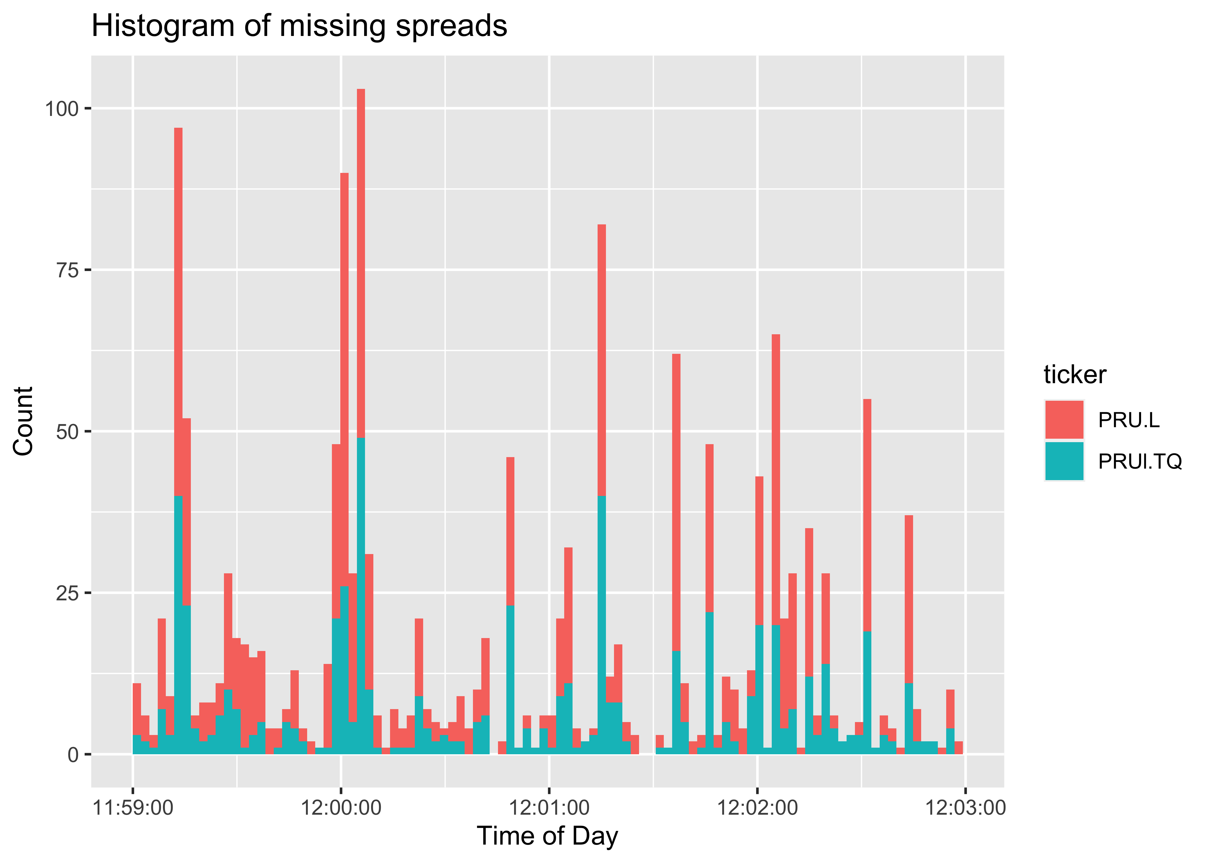
Liquidity measures
With all the data preparation done, we are ready for the actual liquidity measurement. For comparisons across stocks, it is useful to relate the nominal spread to the fundamental value of the security. This is done by the relative quoted bid-ask spread, defined as \(\text{quoted}\_\text{spread}^{rel} = (P^A - P^B)/M\), where \(M\) is the midpoint (also known as the midprice; defined as the average of the best bid and the best ask prices). One can argue that the midpoint is not always representative of the fundamental value, but it has the strong advantage that it is continuously available in the quote data.
# Fundamental value
quotes[, midpoint := (bid_price + ask_price) / 2]
tv_quotes <- tv_quotes |>
mutate(midpoint = (bid_price + ask_price) / 2)The quoted spread can also be measured relative to the tick size. In an open market, the spread can never be below one tick. A tick refers to the tick size of a security. It is the minimum price increment a security can be quoted and traded. The tick size in the example data is half a cent at both exchanges. We refer to the average number of ticks in the bid-ask spread as the tick spread, \(quoted\_spread^{tic} = (P^A - P^B) / tick\_size\).
tick_size <- 0.5Another dimension of quoted liquidity is the market depth. We measure the average depth quoted at the best bid and ask prices. It is defined as \(\text{quoted}\_\text{depth} = (Q^A + Q^B)/2\), where \(Q^A\) and \(Q^B\) are the depths available at the bid and ask prices.
In the code below, we store the liquidity measures in a new data.table named quotes_liquidity. This is because the new variables are averages, observed on a ticker-date frequency, as opposed to the tick-by-tick frequency of the quotes object. We multiply the quoted spread by 10,000 to express it in basis points, and divide the quoted depth by 100,000 to express it in thousand GBP.
The output shows that the liquidity is higher at the LSE than at the TQE. Both in nominal and relative terms, the spreads are somewhat tighter at the LSE, and there is more than three times more depth posted at the LSE.
# Measure the average quote-based liquidity
# This step calculates the mean of each of the market quality variables, for each
# ticker-day (as indicated in `by = c("ticker", "date")`)

quotes_liquidity <- quotes[, {
    quoted_spread = ask_price - bid_price
    list(quoted_spread_nom = mean(quoted_spread, na.rm = TRUE),
         quoted_spread_relative = mean(quoted_spread / midpoint, na.rm = TRUE),
         quoted_spread_tick = mean(quoted_spread / tick_size, na.rm = TRUE),
         quoted_depth = mean(bid_depth * bid_price + ask_depth * ask_price,
                             na.rm = TRUE) / 2)},
    by = c("ticker", "date")]

# Output the liquidity measures, averaged across the five trading days for each ticker.
quotes_liquidity[,
    list(quoted_spread_nom = round(mean(quoted_spread_nom), digits = 2),
         quoted_spread_relative = round(mean(quoted_spread_relative) * 1e4, digits = 2),
         quoted_spread_tick = round(mean(quoted_spread_tick), digits = 2),
         quoted_depth = round(mean(quoted_depth) * 1e-5, digits = 2)),
    by = "ticker"]
ticker quoted_spread_nom quoted_spread_relative quoted_spread_tick
1: PRU.L 0.83 5.65 1.67
2: PRUl.TQ 1.02 6.94 2.05
quoted_depth
1: 24.72
2: 6.65tv_quotes_liquidity <- tv_quotes |>
mutate(quoted_spread = ask_price - bid_price) |>
group_by(ticker, date) |>
summarize(quoted_spread_nom = mean(quoted_spread, na.rm = TRUE),
quoted_spread_relative = mean(quoted_spread / midpoint, na.rm = TRUE) * 1e4,
quoted_spread_tick = mean(quoted_spread / tick_size, na.rm = TRUE),
quoted_depth = mean(bid_depth * bid_price + ask_depth * ask_price,
na.rm = TRUE) / 2 * 1e-5,
.groups = "drop")
tv_quotes_liquidity |>
group_by(ticker) |>
summarize(across(contains("quoted"),
~round(mean(.), digits = 2))) |>
pivot_longer(-ticker) |>
pivot_wider(names_from = name, values_from = value) |>
as_tibble()# A tibble: 2 × 5
ticker quoted_depth quoted_spread_nom quoted_spread_relative
<chr> <dbl> <dbl> <dbl>
1 PRU.L 24.7 0.83 5.65
2 PRUl.TQ 6.65 1.02 6.94
# ℹ 1 more variable: quoted_spread_tick <dbl>Duration-weighted liquidity
The output above are straight averages, implying an assumption that all quote observations are equally important. But whereas some quotes remain valid for several minutes, many don’t last longer than a split-second. For this reason, it is common to either sample the quote data in fixed time intervals (such as at the end of each second), or to weight the observations by their duration. The duration is the time that a quote observation is in force. That is, the time elapsed until the next quote update arrives. We show the duration-weighted approach in the code below (for guidance on how to get the quotes at the end of each second, see Section 3.1).
Note that the duration variable is obtained separately for each ticker and date. Even if we are interested in the average liquidity across dates, it is important to partition by each ticker and date to avoid that duration is calculated overnight (resulting in a huge weight with negative sign, because it will be roughly the opening time minus the closing time). Except for replacing the mean function with the weighted.mean, the code below is very similar to that above.
In the output, we note that the differences between the duration-weighted and the equal-weighted liquidity averages are small. Nevertheless, we consider the duration-weighted average more appropriate because it is not sensitive to short-lived price and depth fluctuations.
# Calculate quote durations
quotes[, duration := c(diff(time), 0), by = c("ticker", "date")]

# Measure the duration-weighted average quote-based liquidity
# The specified subset excludes quotes for which no duration can be calculated
quotes_liquidity_dw <- quotes[!is.na(duration), {
    quoted_spread = ask_price - bid_price
    list(quoted_spread_nom = weighted.mean(quoted_spread,
                                           w = duration, na.rm = TRUE),
         quoted_spread_rel = weighted.mean(quoted_spread / midpoint,
                                           w = duration, na.rm = TRUE),
         quoted_spread_tic = weighted.mean(quoted_spread / tick_size,
                                           w = duration, na.rm = TRUE),
         quoted_depth = weighted.mean(bid_depth * bid_price + ask_depth * ask_price,
                                      w = duration, na.rm = TRUE) / 2)},
    by = c("ticker", "date")]

# Output liquidity measures, averaged across the five trading days for each ticker
quotes_liquidity_dw[,
    list(quoted_spread_nom = round(mean(quoted_spread_nom), digits = 2),
         quoted_spread_rel = round(mean(quoted_spread_rel) * 1e4, digits = 2),
         quoted_spread_tic = round(mean(quoted_spread_tic), digits = 2),
         quoted_depth = round(mean(quoted_depth) * 1e-5, digits = 2)),
    by = "ticker"]
ticker quoted_spread_nom quoted_spread_rel quoted_spread_tic quoted_depth
1: PRU.L 0.84 5.70 1.68 25.65
2: PRUl.TQ 0.99 6.69 1.97 7.06tv_quotes <- tv_quotes |>
group_by(ticker, date) |>
mutate(duration = c(diff(time), 0)) |>
ungroup()
tv_quotes_liquidity <- tv_quotes |>
mutate(quoted_spread = ask_price - bid_price) |>
group_by(ticker, date) |>
summarize(quoted_spread_nom = weighted.mean(quoted_spread, w = duration, na.rm = TRUE),
quoted_spread_relative = weighted.mean(quoted_spread / midpoint, w = duration, na.rm = TRUE) * 1e4,
quoted_spread_tick = weighted.mean(quoted_spread / tick_size, w = duration, na.rm = TRUE),
quoted_depth = weighted.mean(bid_depth * bid_price + ask_depth * ask_price, w = duration, na.rm = TRUE) / 2 * 1e-5,
.groups = "drop")
tv_quotes_liquidity |>
group_by(ticker) |>
summarize(across(contains("quoted"),
~round(mean(.), digits = 2))) |>
pivot_longer(-ticker) |>
pivot_wider(names_from = name, values_from = value) |>
as_tibble()# A tibble: 2 × 5
ticker quoted_depth quoted_spread_nom quoted_spread_relative
<chr> <dbl> <dbl> <dbl>
1 PRU.L 25.6 0.84 5.7
2 PRUl.TQ 7.06 0.99 6.69
# ℹ 1 more variable: quoted_spread_tick <dbl>Consolidated liquidity in fragmented markets
With the competition between exchanges, liquidity is dispersed across venues. For example, if there is a change to the market structure at the LSE, it is typically not sufficient to analyze liquidity at LSE alone. If liquidity is reduced at the LSE, it may simultaneously be boosted at the TQE. To assess the overall market quality, which may be most relevant for welfare, it is often necessary to consider the consolidated liquidity.
In Europe, the consolidated liquidity is sometimes referred to as the European Best Bid and Offer (EBBO). The terminology follows in the footsteps of the US market, where the National Best Bid and Offer (NBBO) is transmitted to the market on continuous basis. To obtain the EBBO, one needs to merge the LOB data from each relevant venue, and then determine the EBBO prices and depths. In the code below, we show step-by-step how to do that.
Retaining only the last quote update in each interval
Quote updates tend to cluster and it is common that several observations have identical timestamps. Multiple observations at one timestamp can be due to several investors responding to the same events, or that one market order leads to several LOB updates as it is executed against multiple limit orders. When matching quotes across venues, we need to restrict the number of observations per unit of time to one. There is no sensible way to distinguish observations with identical timestamps. In lack of a better approach, we retain the last observation in each interval.
# Retain only the last observation per unit of time
# The function `duplicated` returns `TRUE` if the observation is a duplicate of another
# observation based on the columns given in the `by` option, and `FALSE` otherwise.
# The option `fromLast = TRUE` ensures that the last rather than the first observation
# in each millisecond that returns `FALSE`.
quotes <- quotes[!duplicated(quotes, fromLast = TRUE, by = c("ticker", "date", "time"))]
tv_quotes <- tv_quotes |>
group_by(ticker, date, time) |>
slice(n()) |>
ungroup() |>
lazy_dt()Merging quotes from different venues
We are now ready to match the quotes from the two exchanges. First, we create separate quote data sets for the two exchanges. Second, we merge the two by matching on date and time. Third, we forward-fill quotes from both venues, such that for each LSE quote we know the prevailing TQE quote, and vice versa. The validity of this is ensured by the option sort = TRUE in the merge function, which returns a data.table that is sorted on the matching variables.
# Merge quotes from two venues trading the same security
# In the `merge` function, we add exchange suffixes to the variable names to keep track of
# which quote comes from which exchange, using the option `suffixes`.
# The option `all = TRUE` specifies that unmatched observations from both sets of quotes
# should be retained (known as an outer join).
venues <- c("_lse", "_tqe")

quotes_lse <- quotes[ticker == "PRU.L", .SD, .SDcols = c("date", "time", lob_variables)]
quotes_tqe <- quotes[ticker == "PRUl.TQ", .SD, .SDcols = c("date", "time", lob_variables)]

quotes_ebbo <- merge(quotes_lse, quotes_tqe,
                     by = c("date", "time"),
                     suffixes = venues,
                     all = TRUE, sort = TRUE)
Next, we forward-fill the quoted prices and depth for each exchange.
local_lob_variables <- paste0(lob_variables, rep(venues, each = 4))

quotes_ebbo[, (local_lob_variables) := lapply(.SD, nafill, type = "locf"),
  .SDcols = (local_lob_variables),
    by = "date"]
tv_quotes_ebbo <- tv_quotes |>
select(-midpoint, -duration) |>
mutate(ticker = case_when(ticker == "PRUl.TQ" ~ "tqe",
ticker == "PRU.L" ~ "lse")) |>
pivot_wider(names_from = ticker,
values_from = matches("bid|ask")) |>
arrange(date, time)
tv_quotes_ebbo <- tv_quotes_ebbo |>
group_by(date) |>
fill(matches("bid|ask")) |>
ungroup()The best bid price at each point in time is the maximum of the best bid at the LSE and the best bid at the TQE. Similarly, the best ask is the minimum of the best ask prices at the two venues. We calculate the best bid using the parallel maxima function, pmax, which returns the highest value in each row. The best ask is obtained in the same way, using the parallel minima function, pmin.
Note that it would also be possible to obtain the EBBO using a for loop, checking row-wise which is the highest bid and lowest ask. When working with large data sets in R, however, loops become extremely slow. It is strongly encouraged to run vectorised operations for the whole column at once (like we do here), or to apply functions repeatedly to blocks of data (like we have done several times above).
We obtain the depth at the best prices by summing the depth of the individual venues. When doing this, we should only consider both venues at times when they are both at the best price. When the two venues have the same best bid, for example, we calculate the consolidated bid depth as the sum of the two. To code this, we use the feature that a logical variable (with values FALSE or TRUE; such as bid_price_lse == best_bid_price) works as a binary variable (with values 0 or 1) when used in multiplication.
# Obtain the EBBO prices and depths
quotes_ebbo[, best_bid_price := pmax(bid_price_lse, bid_price_tqe, na.rm = TRUE)]
quotes_ebbo[, best_ask_price := pmin(ask_price_lse, ask_price_tqe, na.rm = TRUE)]
quotes_ebbo[, best_bid_depth := bid_depth_lse * (bid_price_lse == best_bid_price) +
              bid_depth_tqe * (bid_price_tqe == best_bid_price)]
quotes_ebbo[, best_ask_depth := ask_depth_lse * (ask_price_lse == best_ask_price) +
              ask_depth_tqe * (ask_price_tqe == best_ask_price)]
Finally, we drop local exchange variables and objects
quotes_ebbo[, (local_lob_variables) := NULL]
rm(quotes_lse, quotes_tqe, quotes, local_lob_variables)
tv_quotes_ebbo <- tv_quotes_ebbo |>
mutate(best_bid_price = pmax(bid_price_lse, bid_price_tqe, na.rm = TRUE),
best_ask_price = pmin(ask_price_lse, ask_price_tqe, na.rm = TRUE),
best_bid_depth = bid_depth_lse * (bid_price_lse == best_bid_price) +
bid_depth_tqe * (bid_price_tqe == best_bid_price),
best_ask_depth = ask_depth_lse * (ask_price_lse == best_ask_price) +
ask_depth_tqe * (ask_price_tqe == best_ask_price)
)Finally, we drop local exchange variables and objects
tv_quotes_ebbo <- tv_quotes_ebbo |>
  select(date, time, contains("best")) |>
  lazy_dt()
Fundamental value
We can now obtain EBBO midpoints, as a proxy of fundamental value that factors in liquidity posted at multiple exchanges.
# Calculate EBBO midpoints
quotes_ebbo[, midpoint := (best_bid_price + best_ask_price) / 2]
tv_quotes_ebbo <- tv_quotes_ebbo |>
mutate(midpoint = (best_bid_price + best_ask_price) / 2)Screening
As above, we check that the EBBO quotes are economically meaningful by tabulating the counts of nominal spread levels. This exercise shows us that the consolidated spread is not strictly positive. There are numerous cases of zeroes, known as locked quotes, and also many negatives, referred to crossed quotes. This is possible because orders at the LSE and the TQE are never executed against each other – it takes arbitrageurs to step in and act on crossed markets. Locked and crossed spreads are not uncommon in consolidated data. For an analysis of the incidence in US markets, see Shkilko, van Ness & van Ness, 200814.
It is also notable from the table that the maximum consolidated spread is 2.5, as compared to the spreads of up to 11 recorded in the single-venue analysis. By definition, the EBBO quoted spread is never wider than at the single venues.
# Output an overview of the EBBO nominal quoted bid-ask spread
table(quotes_ebbo$best_ask_price - quotes_ebbo$best_bid_price)
    -1   -0.5      0    0.5      1    1.5      2    2.5    3.5
     2    127   6367 104351 103265   4668    637     51      1
tv_quotes_ebbo |>
transmute(ebbo_nominal_spread = best_ask_price - best_bid_price) |>
count(ebbo_nominal_spread) |>
as_tibble()# A tibble: 9 × 2
ebbo_nominal_spread n
<dbl> <int>
1 -1 2
2 -0.5 127
3 0 6367
4 0.5 104351
5 1 103265
6 1.5 4668
7 2 637
8 2.5 51
9 3.5 1Observations with locked or crossed quotes are usually excluded when measuring market quality. It is also common to exclude bid-ask spread observations that are unrealistically high. We have no such cases in this sample, but, for illustration, we include a filter that would capture spreads that relative to the share price are wider than 5%.
threshold <- 0.05In the procedure below, we flag the problematic quotes, but we do not exclude them. If they were deleted, it would imply that the last observation before the excluded spread was still in force, which may mislead subsequent analysis.
The output shows that 2.90% of the quote observations are locked, while 0.06% are crossed.
# Flag problematic consolidated quotes
quotes_ebbo[, c("crossed", "locked", "large") := {
    quoted_spread = (best_ask_price - best_bid_price)
    list(quoted_spread < 0, quoted_spread == 0, quoted_spread / midpoint > threshold)}]

# Count the incidence of the consolidated quote flags
quotes_ebbo_filters  <- quotes_ebbo[,
    list(crossed = mean(crossed, na.rm = TRUE),
         locked = mean(locked, na.rm = TRUE),
         large = mean(large, na.rm = TRUE))]

# Output the fraction of quotes that is flagged
quotes_ebbo_filters[,
    lapply(.SD * 100, round, digits = 2), .SDcols = c("crossed", "locked", "large")]
crossed locked large
1: 0.06 2.9 0tv_quotes_ebbo <- tv_quotes_ebbo |>
mutate(quoted_spread = best_ask_price - best_bid_price,
crossed = quoted_spread < 0,
locked = quoted_spread == 0,
large = quoted_spread / midpoint > threshold) |>
lazy_dt()
tv_quotes_ebbo |>
summarize(across(c(crossed, locked, large),
~round(100 * mean(.),2))) |>
as_tibble()# A tibble: 1 × 3
crossed locked large
<dbl> <dbl> <dbl>
1 0.06 2.9 0Consolidated liquidity measures
We obtain duration-weighted measures of consolidated liquidity in the same way as above. The only difference here is that we subset the quotes to filter out crossed and locked markets.
The consolidated relative quoted bid-ask spread is 5.59 basis points, as compared to 5.70 and 6.69 basis points at LSE and TQE locally. The consolidated depth, 3.14 million GBP, is somewhat lower than the sum of the local depths seen above. This is to be expected, as some of the local depth is posted at price levels that are inferior to the EBBO.
# Measure the duration-weighted consolidated quotes liquidity
# Because this is the EBBO, there is no variation across tickers, but different averages
# across dates are considered
quotes_ebbo[, duration := c(diff(time), 0), by = "date"]

# Note that the subset used here excludes crossed and locked quotes
quotes_liquidity_ebbo_dw <- quotes_ebbo[!crossed & !locked & !large, {
    quoted_spread = best_ask_price - best_bid_price

    list(quoted_spread_nom = weighted.mean(quoted_spread,
                                           w = duration, na.rm = TRUE),
         quoted_spread_relative = weighted.mean(quoted_spread / midpoint,
                                           w = duration, na.rm = TRUE),
         quoted_spread_tick = weighted.mean(quoted_spread / tick_size,
                                           w = duration, na.rm = TRUE),
         quoted_depth = weighted.mean(best_bid_depth * best_bid_price +
                                      best_ask_depth * best_ask_price,
                                      w = duration, na.rm = TRUE) / 2)},
    by = "date"]

# Output the liquidity measures, averaged across the five trading days
quotes_liquidity_ebbo_dw[,
    list(quoted_spread_nom = round(mean(quoted_spread_nom), digits = 2),
         quoted_spread_relative = round(mean(quoted_spread_relative * 1e4), digits = 2),
         quoted_spread_tick = round(mean(quoted_spread_tick), digits = 2),
         quoted_depth = round(mean(quoted_depth * 1e-6), digits = 2))]
quoted_spread_nom quoted_spread_relative quoted_spread_tick quoted_depth
1: 0.82 5.59 1.65 3.14tv_quotes_ebbo <- tv_quotes_ebbo |>
group_by(date)|>
mutate(duration = c(diff(time), 0)) |>
ungroup()
tv_quotes_liquidity_ebbo_dw <- tv_quotes_ebbo |>
group_by(date) |>
mutate(quoted_spread = best_ask_price - best_bid_price) |>
filter(!crossed, !locked, !large) |>
summarize(quoted_spread_nom = weighted.mean(quoted_spread, w = duration, na.rm = TRUE),
quoted_spread_relative = weighted.mean(quoted_spread / midpoint, w = duration, na.rm = TRUE) * 1e4,
quoted_spread_tick = weighted.mean(quoted_spread / tick_size, w = duration, na.rm = TRUE),
quoted_depth = weighted.mean(best_bid_depth * best_bid_price + best_ask_depth * best_ask_price, w = duration, na.rm = TRUE) / 2 * 1e-5)
tv_quotes_liquidity_ebbo_dw |>
summarize(across(contains("quoted"),
~round(mean(.), digits = 2))) |>
as_tibble()# A tibble: 1 × 4
quoted_spread_nom quoted_spread_relative quoted_spread_tick quoted_depth
<dbl> <dbl> <dbl> <dbl>
1 0.82 5.59 1.65 31.4Data export
As we will reuse the consolidated quotes in the applications below, we save the quotes_ebbo object to disk.
We export the consolidated quotes using fwrite.
fwrite(quotes_ebbo, file = "quotes_ebbo.csv")We export the consolidated quotes using write_csv.
write_csv(as_tibble(tv_quotes_ebbo), file = "tv_quotes_ebbo.csv")Trade-based liquidity
A shortcoming of the quoted bid-ask spread is that it can only be measured for liquidity that is visible in the quote data. That is not always the full picture. For example, limit order books typically allow hidden liquidity, and dealers often offer price improvements on their quotes. Outside the exchanges, trades execute extensively at venues without quotes, such as dark pools. The effective bid-ask spread is a good alternative because it uses the trade price (the effective price) instead of the quoted price, and benchmarks it to the spread midpoint holding at the time of the trade.
Whenever there is a trade, the price tends to move in the direction of the trade. This is known as price impact, and is an aspect of market depth. Whereas the quoted depth measure above captures depth in a mechanic sense (how much can you trade without changing the price), price impact also captures other traders’ response to a trade. The response may be either that the LOB is refilled (if the trade is viewed as uninformative), or that liquidity is withdrawn (if the trade is viewed as a signal of more to come).
For the market makers, who makes a living from the bid-ask spread, price impact undermines the profits. A more relevant measure for them may be the realized spread, which accounts for price impact by evaluating the trade price relative to the midpoint some time later. The three trade-based liquidity measures are closely related: the realized spread equals the effective spread minus the price impact.
Trade data inspection and preparation
We load the trade data and view the data structure. The ticker, date, and time variables follow the same structure as in quotes data, so we can proceed with the same date and time transformations as above.
trades_url <- "http://tinyurl.com/prutrades"There are three more variables: Price, Volume, and MMT Classification. As discussed above, we refer to the number of shares executed in a trade as “size” (we reserve the term “volume” to the sum of trade sizes in a given interval). We rename the Volume variable accordingly, and also alter the other variable names to make them easier to work with in R.
# Load the trade data
trades <- fread(trades_url)

# View the trade data
trades
#RIC Domain Date-Time GMT Offset Type Price Volume
1: PRU.L Market Price 2021-06-07 07:00:09 1 Trade 1481.5 11379
2: PRU.L Market Price 2021-06-07 07:00:12 1 Trade 1477.5 703
3: PRU.L Market Price 2021-06-07 07:00:12 1 Trade 1477.5 327
4: PRU.L Market Price 2021-06-07 07:00:12 1 Trade 1477.5 650
5: PRU.L Market Price 2021-06-07 07:00:12 1 Trade 1478.0 327
---
34513: PRUl.TQ Market Price 2021-06-11 15:28:56 1 Trade 1492.0 315
34514: PRUl.TQ Market Price 2021-06-11 15:28:56 1 Trade 1491.5 50
34515: PRUl.TQ Market Price 2021-06-11 15:28:56 1 Trade 1491.5 170
34516: PRUl.TQ Market Price 2021-06-11 15:28:58 1 Trade 1492.0 6
34517: PRUl.TQ Market Price 2021-06-11 15:29:06 1 Trade 1492.0 9
Exch Time MMT Classification
1: 07:00:09.478177000 1O-------P----
2: 07:00:12.859753000 12-------PH---
3: 07:00:12.859753000 12-------PH---
4: 07:00:12.859753000 12-------PH---
5: 07:00:12.860655000 12-------PH---
---
34513: 15:28:56.202000000 12-------PH---
34514: 15:28:56.218000000 12-------PH---
34515: 15:28:56.413000000 12-------PH---
34516: 15:28:58.062128000 32D---S--PH---
34517: 15:29:06.141081000 32D---S--PH---# Rename the variables
raw_trade_variables <- c("#RIC", "Date-Time", "Exch Time", "GMT Offset",
"Price", "Volume", "MMT Classification")
new_trade_variables <- c("ticker", "date_time", "exchange_time", "gmt_offset",
"price", "size", "mmt")
setnames(trades,
old = raw_trade_variables,
new = new_trade_variables)Finally, we remove the columns Domain and Type.
trades[, c("Domain", "Type") := NULL]tv_trades <- read_csv(trades_url, col_types = list(`Exch Time` = col_character()))
tv_trades <- lazy_dt(tv_trades)The raw data looks as follows.
tv_tradesSource: local data table [34,517 x 9]
Call: `_DT17`
`#RIC` Domain `Date-Time` `GMT Offset` Type Price Volume `Exch Time`
<chr> <chr> <dttm> <dbl> <chr> <dbl> <dbl> <chr>
1 PRU.L Market… 2021-06-07 07:00:09 1 Trade 1482. 11379 07:00:09.4…
2 PRU.L Market… 2021-06-07 07:00:12 1 Trade 1478. 703 07:00:12.8…
3 PRU.L Market… 2021-06-07 07:00:12 1 Trade 1478. 327 07:00:12.8…
4 PRU.L Market… 2021-06-07 07:00:12 1 Trade 1478. 650 07:00:12.8…
5 PRU.L Market… 2021-06-07 07:00:12 1 Trade 1478 327 07:00:12.8…
6 PRU.L Market… 2021-06-07 07:00:12 1 Trade 1478 201 07:00:12.8…
# ℹ 34,511 more rows
# ℹ 1 more variable: `MMT Classification` <chr>
# Use as.data.table()/as.data.frame()/as_tibble() to access resultsWe rename the variables.
tv_trades <- tv_trades |>
  rename(ticker = `#RIC`,
         date_time = `Date-Time`,
         gmt_offset = `GMT Offset`,
         price = Price,
         size = Volume,
         exchange_time = `Exch Time`,
         mmt = `MMT Classification`
  ) |>
  select(-c("Domain", "Type"))
Dates and timestamps
As above, we filter out the first and last minute of continuous trading, as well as the minutes surrounding the intraday auction. Note here that filtered trades are excluded, not just set as missing. This is OK, because we won’t do any forward-filling for the trade data.
# Extract dates
trades[, date := as.Date(date_time)]

# Convert time stamps to numeric format, expressed in seconds past midnight
trades[, time := {
    time_elements = strsplit(exchange_time, split = ":")
    time_elements = do.call(rbind, time_elements)
    time = as.numeric(time_elements[, 1]) * 3600 +
      as.numeric(time_elements[, 2]) * 60 +
      as.numeric(time_elements[, 3]) +
      gmt_offset * 3600
    list(time)}]

# Delete raw time variables
trades[, c("date_time", "exchange_time", "gmt_offset") := NULL]

# Retain trades from the continuous trading sessions
trades <- trades[time > (open_time + 60) & time < (close_time - 60) &
                    (time < (intraday_auction_time - 60) |
                     time > (intraday_auction_time + 3 * 60))]
tv_trades <- tv_trades |>
separate(exchange_time,
into = c("hour", "minute", "second"),
sep=":",
convert = TRUE) |>
mutate(date = as.Date(date_time),
time = hour * 3600 + minute * 60 + second + gmt_offset * 3600)Having made sure that dates and times are in the desired format, we can save space by dropping the raw time and date variables. Further, we only retain trades from the continuous trading sessions.
tv_trades <- tv_trades|>
  select(-c("date_time", "gmt_offset","hour","minute","second"))

tv_trades <- tv_trades |>
  filter(time > hms::as_hms("08:01:00"),
         time < hms::as_hms("16:29:00"),
         time < hms::as_hms("11:59:00") | time > hms::as_hms("12:03:00")) |>
  lazy_dt()
Trade variables
A line plot offers a good overview of price data. In the figure below, we see that the trade prices are plagued by outliers that seem to be close to zero. The out-of-sequence prices are recorded on all trading dates and at virtually all times of the day. These outliers need to be addressed before we can proceed with the analysis.
# Plot the trade prices
trades |>
  ggplot(aes(x = time, y = price)) +
  geom_line() +
  facet_wrap(~date, ncol= 1) +
  labs(title = "Trade prices",  y = "Price", x = "Time (seconds past midnight)")
tv_trades |>
  as_tibble() |>
  ggplot(aes(x = hms::hms(time), y = price)) +
  geom_line() +
  facet_wrap(~date, ncol= 1) +
  labs(title = "Trade prices",  y = "Price", x = "Time (seconds past midnight)")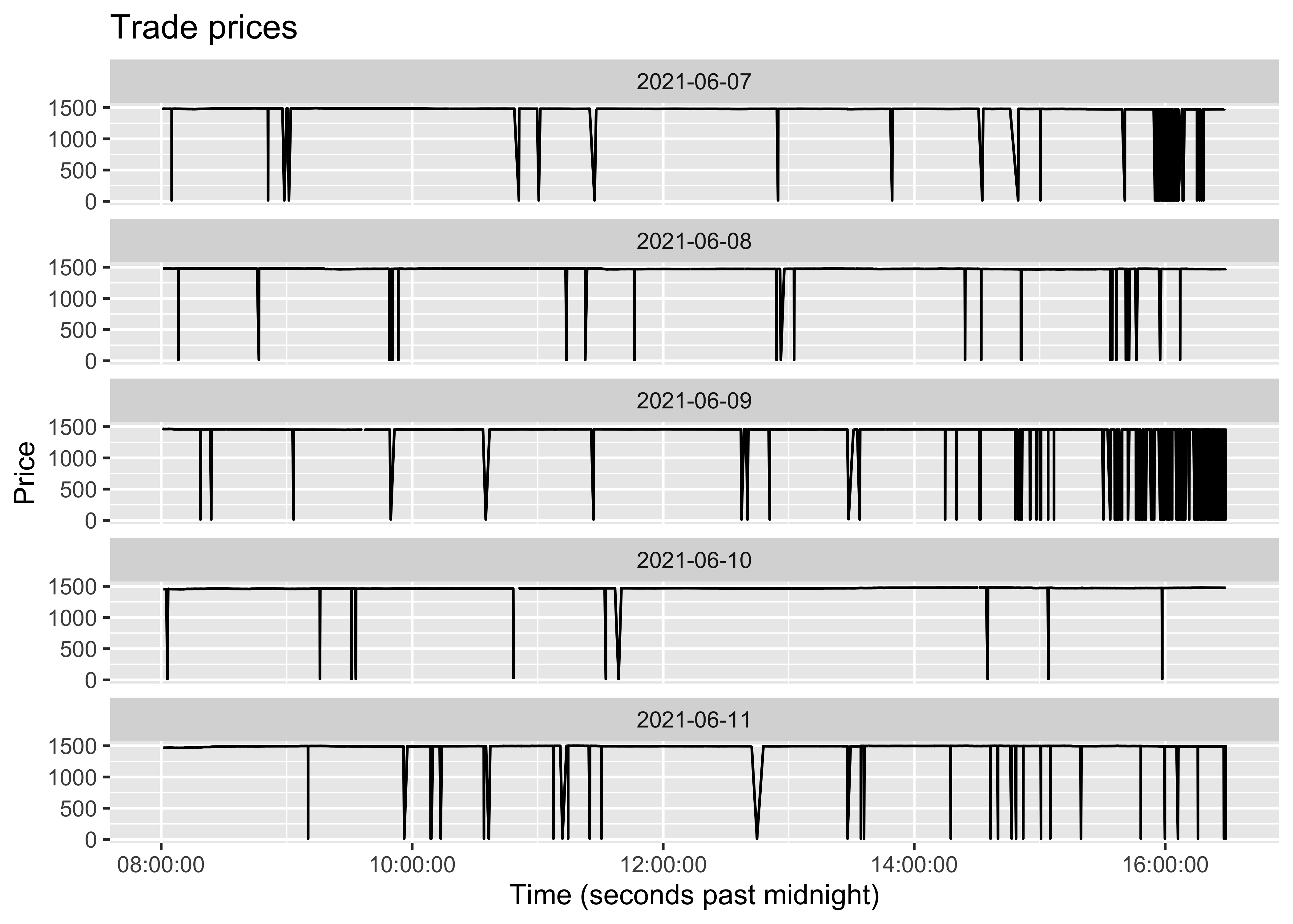
There are various ways to handle outliers, but the best way is to understand them. In trade data sets, there is often information provided about the trade circumstances (for quote observations, such information is often sparse). In the current data set, the best piece of supporting information is the MMT code. MMT, short for Market Model Typology, is a rich set of flags reported for trades in Europe in recent years. For details, see the website of the Fix Trading Community.
The MMT code is a 14-character string, where each position corresponds to one flag. The first character specifies the type of market mechanism. For example, “1” tells us that the trade was recorded in an LOB market, “3” indicates dark pools, “4” is for off-book trading, and “5” is for periodic auctions. The second character indicates the trading mode, where, for example, continuous trading is indicated by “2”.
An overview of the populated values shows in the first column that the LOB market with continuous trading (“12”) is by far the most common combination remaining after applying the filters above, followed by dark pool continuous trading (“32”).
The low-priced trades are captured in the second column. All those trades are off-book, as indicated by the first digit being “4”. The second digit holds information about how the off-book trades are reported (“5” is for on-exchange, “6” is for off-exchange, and “7” indicates systematic internalisers).
# Output an overview of the MMT codes
# The function `substr` is used here to extract the first two characters of the MMT code
table(substr(trades[, mmt], start = 1, stop = 2), trades[, price] < 100)
     FALSE  TRUE
  12 27737     0
  32  3383     0
  3U   114     0
  45  1221    28
  46     0    41
  47  1023   236
  5U    88     0
tv_trades |>
mutate(message = str_extract(mmt, "^.{2}")) |>
mutate(small_price = price < 100) |>
count(message, small_price)Source: local data table [10 x 3]
Call: copy(`_DT18`)[, `:=`(message = str_extract(mmt, "^.{2}"))][,
`:=`(small_price = price < 100)][, .(n = .N), keyby = .(message,
small_price)]
message small_price n
<chr> <lgl> <int>
1 12 FALSE 27737
2 32 FALSE 3383
3 3U FALSE 114
4 45 NA 4
5 45 FALSE 1221
6 45 TRUE 28
# ℹ 4 more rows
# Use as.data.table()/as.data.frame()/as_tibble() to access resultsIn this analysis we are focusing on liquidity at the exchanges. Accordingly, we use the MMT codes to filter out trades from other trading venues. Restricting the trades to continuous trading at the exchanges, we obtain price plots that are free from outliers.
# Define a subset with continuous trades only
LOB_continuous_trades <- substr(trades[, mmt], start = 1, stop = 2) == "12"

# Plot the prices of continuous trades
ggplot(trades[LOB_continuous_trades],
       aes(x = time, y = price)) +
  geom_line() +
  facet_wrap(~date, ncol = 1) +
  labs(title = "Trade prices", y = "Price", x = "Time (seconds past midnight)")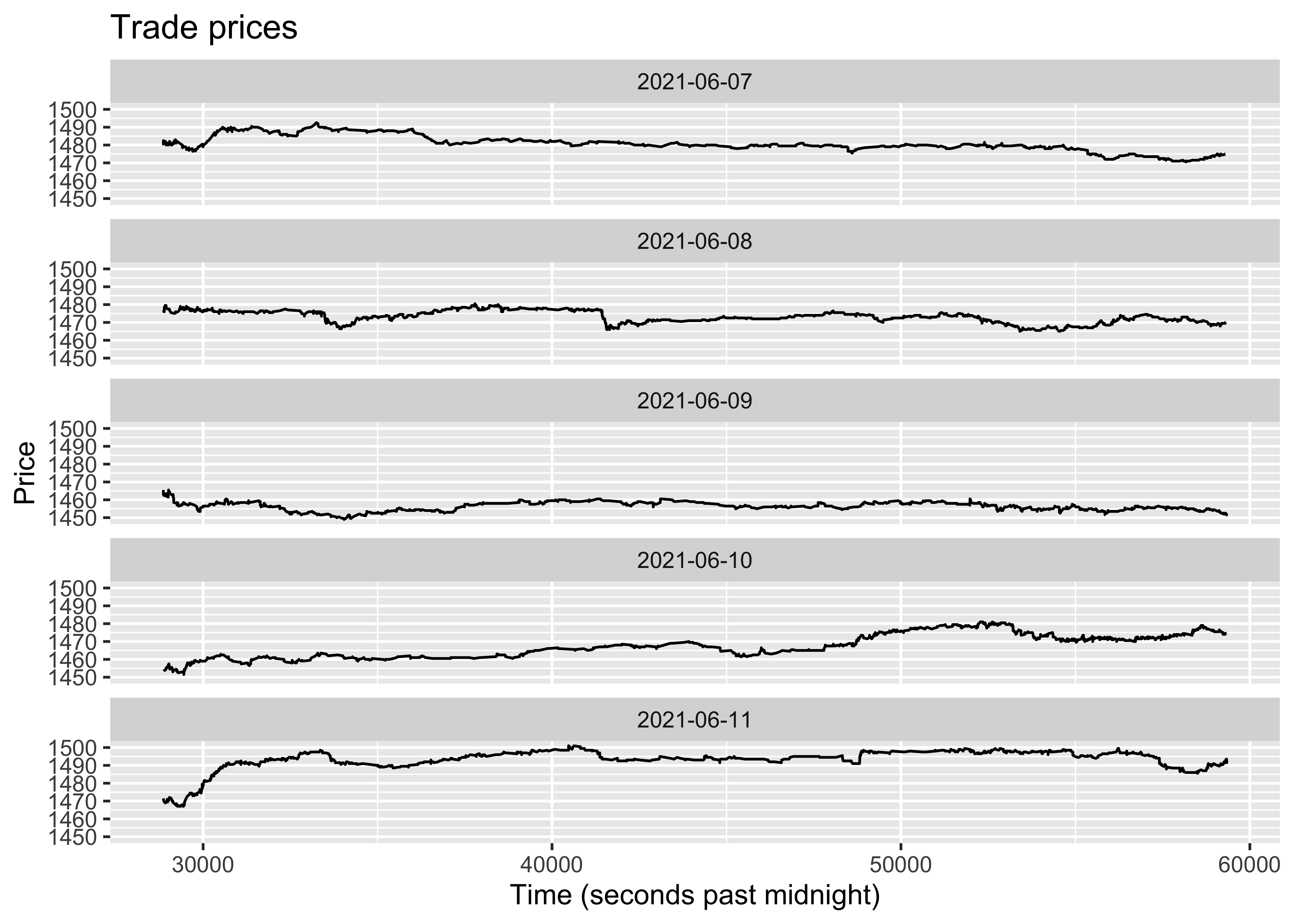
tv_trades |>
  filter(str_extract(mmt, "^.{2}") == "12") |>
  as_tibble() |>
  ggplot(aes(x = hms::hms(time), y = price)) +
  geom_line() +
  facet_wrap(~date, ncol = 1) +
  labs(title = "Trade prices", y = "Price", x = "Time (seconds past midnight)")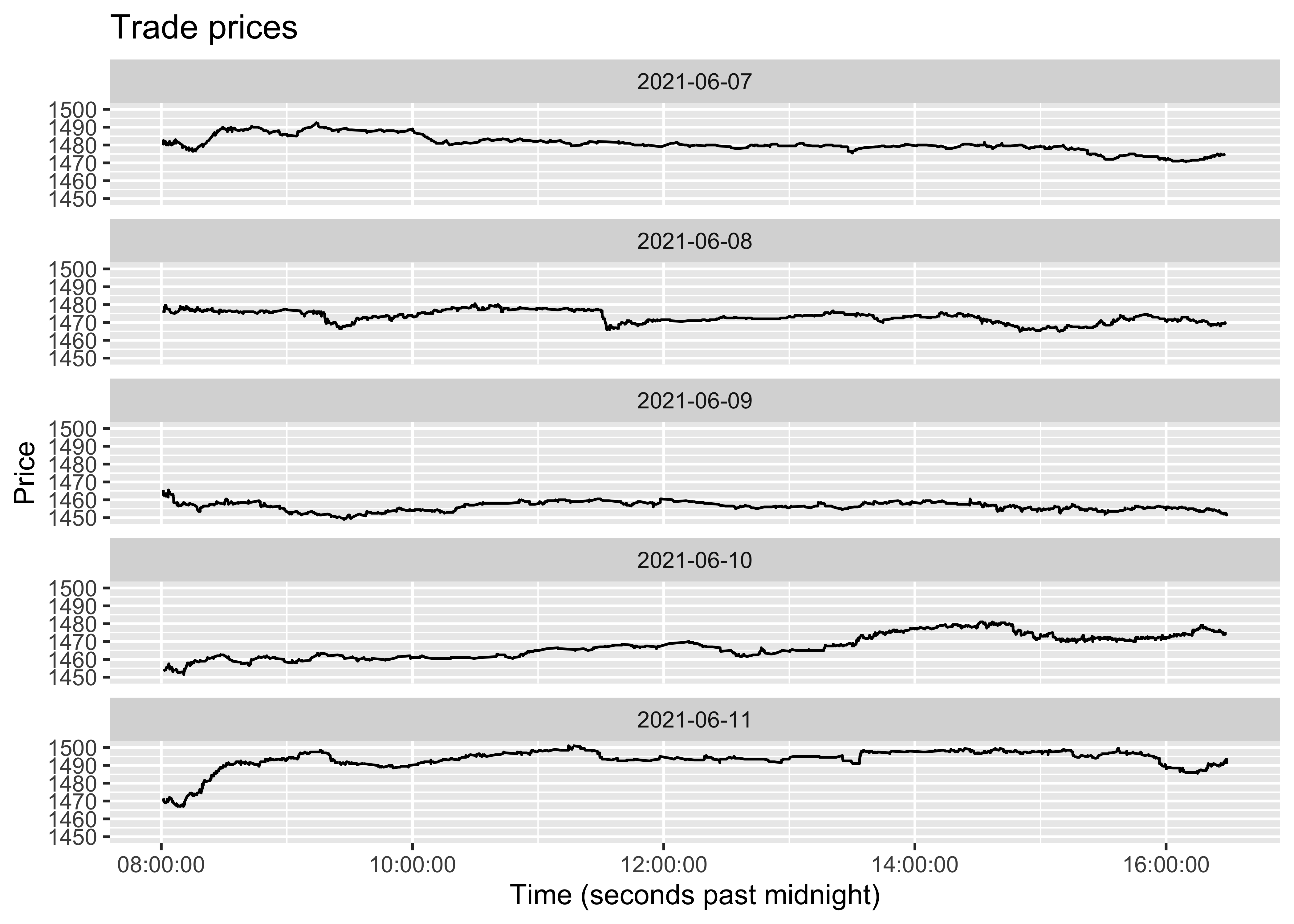
Further detective work reveals that the trade price outliers are not erroneous, they are just stated in pounds rather than in pence. This is clear because the outliers are priced 100 times lower than the other trades. Apparently, some off-exchange trades follow a different price reporting convention.
# View trades with low prices
trades[price < 100]
ticker price size mmt date time
1: PRU.L 14.80000 635 47------MP---- 2021-06-07 29102.70
2: PRU.L 14.86625 400 45------MP---- 2021-06-07 31868.09
3: PRU.L 14.86062 204 45------MP---- 2021-06-07 32331.08
4: PRU.L 14.85125 540 45------MP---- 2021-06-07 32466.05
5: PRU.L 14.83875 1042 45------MP---- 2021-06-07 39062.65
---
301: PRU.L 14.88500 1 47------MP---- 2021-06-11 57966.07
302: PRU.L 14.87000 434 47------MP---- 2021-06-11 58540.00
303: PRU.L 14.91500 870 47------MP---- 2021-06-11 59286.00
304: PRU.L 14.92000 1463 46------MP---- 2021-06-11 59336.00
305: PRU.L 14.92000 1463 46------MP---- 2021-06-11 59336.00Quirks in the data are not unusual, and if they go unnoticed they can have strong impact on the market quality measures. The take-away from the outlier analysis is that there is often an explanation for why their prices are off. It is not always as straightforward as here, but it is worthwhile to try to find out what the cause of the deviations is. Other potential explanations are that the time stamps are off (possibly due to delayed reporting) or that the pricing is not done at the market (but in accordance to some derivative contract).
For the analysis below, we want to focus on exchange trades. Accordingly, we filter out all trades that are not from the on-exchange continuous trading sessions.
# Retain continuous LOB trades only
trades <- trades[LOB_continuous_trades]
tv_trades <- tv_trades |>
filter(str_extract(mmt, "^.{2}") == "12")Matching trades to quotes
To evaluate the cost of trading, we want to compare the trade price to the fundamental value at the time of trade, as implied by the bid-ask quotes.
The objective of matching trades and quotes is to obtain the quotes that prevailed just before the trade. This is straightforward in settings where the trades and quotes are recorded at the same point, such that they are correctly sequenced. In other settings, the timestamps may need to be adjusted due to reporting latencies, or the trade size needs to be matched to changes in quoted depth (Jurkatis, 2021)15.
For US data, the most common approach is to match trades to the last quotes available in the millisecond or microsecond before the trade, as prescribed by Holden and Jacobsen (2014)16. There is, however, an active debate which timestamp to use. Several recent papers advocate the use of participant time stamps in trade and quote matching, see references about US timestamps above.
In lack of specific guidance for stocks traded in the UK, we match trades to quotes prevailing just before the trade. Based on the assumption that the combined liquidity from LSE and TQE offers the best fundamental value approximation, we match trades from all venues to the EBBO.
The merge function in data.table can be called as above by merge(dt1, dt2) (for two data.tables named dt1 and dt2), or simply dt1[dt2]. We use the latter approach here because it allows us to specify what to do when the timestamps do not match exactly. The option roll = TRUE specifies that each observation in trades should be matched to the quotes_ebbo observation with the latest timestamp that is equal or earlier than the trade timestamp. However, we don’t want equal matches, because the quote observation should always be before the trade. To avoid matching to contemporaneous quotes, which may be updated to reflect the impact of the trade itself, we add one microsecond to the quote timestamps before running the merge function. For further understanding and illustration of the rolling join, we refer to the blog post by R-Bloggers.
For the sake of completeness, you can load the EBBO quote data which we stored at an intermediate step above as follows.
quotes_ebbo <- fread(file = "quotes_ebbo.csv")# Adjust quote time stamps by one microsecond
setnames(quotes_ebbo, old = "time", new = "quote_time")
quotes_ebbo[, time := quote_time + 0.000001]
# Sort trades and quotes (this specifies the matching criteria for the merge function)
setkeyv(trades, cols = c("date", "time"))
setkeyv(quotes_ebbo, cols = c("date", "time"))
# Match trades to quotes prevailing at the time of trade
# The rolling is done only for the last of the matching variables, in this case "time"
# `mult = "last"` specifies that if there are multiple matches with identical timestamps,
# the last match is retained
trades <- quotes_ebbo[trades, roll = TRUE, mult = "last"]For the sake of completeness, you can load the EBBO quote data which we stored at an intermediate step above as follows.
tv_quotes_ebbo <- read_csv("tv_quotes_ebbo.csv")

tv_quotes_ebbo <- tv_quotes_ebbo |>
  mutate(time = time + 0.000001) |>
  arrange(date, time) |>
  as_tibble()

tv_trades <- tv_trades |>
  arrange(date, time) |>
  as_tibble()

tv_trades <- tv_trades |>
  left_join(tv_quotes_ebbo, join_by(date, closest(time >= time)), suffix = c("", "_quotes")) |>
  lazy_dt()
Further screening
As some trades may be matched to crossed or locked quotes, another round of data screening is required. Because such quotes are not considered reliable, we do not include those trades in the liquidity measurement. Furthermore, if there are trades that could not be matched to any quotes, or that lack information on price or size, they should be excluded too.
The output shows that 88.5% of the trades at LSE are eligible for the liquidity analysis, and 96.8% of the trades at TQE. The criterion that drives virtually all exclusions in the sample is the locked quotes.
# Flag trades that should be included
trades[, include := !crossed & !locked & !large & !is.na(size) & size > 0 &
                    !is.na(price) & price > 0 & !is.na(midpoint) & midpoint > 0]

# Report trade filtering stats
trades_filters <- trades[,
    list(crossed = mean(crossed, na.rm = TRUE),
         locked = mean(locked, na.rm = TRUE),
         large = mean(large, na.rm = TRUE),
         no_price = mean(is.na(price) | price == 0),
         no_size = mean(is.na(size) | size == 0),
         no_quotes = mean(is.na(midpoint) | midpoint <= 0),
         included = mean(include)),
    by = "ticker"]

trades_filters[,
  lapply(.SD * 100, round, digits = 2),
  .SDcols = c("crossed", "locked", "large", "no_price", "no_size", "no_quotes", "included"),
  by = "ticker"]
ticker crossed locked large no_price no_size no_quotes included
1: PRU.L 0.30 11.20 0 0 0 0.00 88.50
2: PRUl.TQ 0.07 3.05 0 0 0 0.02 96.85tv_trades <- tv_trades |>
mutate(include = !crossed & !locked & !large & !is.na(size) & size > 0 &
!is.na(price) & price > 0 & !is.na(midpoint) & midpoint > 0)
trades_filters <- tv_trades |>
group_by(ticker) |>
summarize(
crossed = mean(crossed, na.rm = TRUE),
locked = mean(locked, na.rm = TRUE),
large = mean(large, na.rm = TRUE),
no_price = mean(is.na(price) | price == 0),
no_size = mean(is.na(size) | size == 0),
no_quotes = mean(is.na(midpoint) | midpoint <= 0),
included = mean(include)
)
# Round percentages and display
trades_filters |>
mutate(across(crossed:included, ~round(. * 100, digits = 2))) |>
select(ticker, crossed, locked, large, no_price, no_size, no_quotes, included) |>
as_tibble()# A tibble: 2 × 8
ticker crossed locked large no_price no_size no_quotes included
<chr> <dbl> <dbl> <dbl> <dbl> <dbl> <dbl> <dbl>
1 PRU.L 0.3 11.2 0 0 0 0 88.5
2 PRUl.TQ 0.07 3.05 0 0 0 0.02 96.8Direction of trade
In empirical market microstructure, we often need to determine the direction of trade. If a trade happens following a buy market order, it is said to be buyer-initiated, and vice versa.
The most common tool to determine the direction of trade is the algorithm prescribed by Lee and Ready (1991)17. They primarily recommend the quote rule, saying that a trade is buyer-initiated if the trade price is above the prevailing midpoint, and seller-initiated if it is below. When the price equals the midpoint, Lee and Ready propose the tick rule. It specifies that a trade is buyer-initiated (seller-initiated) if the price is higher (lower) than the closest previous trade with a different price.
The quote rule is straightforward to implement using the sign function, which returns +1 when the price deviation from the midpoint is positive and -1 if it is negative. The tick rule, in contrast, requires several steps of code. We create a new data.table, named price_tick, which in addition to date and time observations for each trade, indicates whether a trade is priced higher (+1), lower (-1), or the same (0) as the previous one. We then exclude all trades that don’t imply a price change. Finally, we merge the price_tick and the trades objects, such that each trade is associated with the latest previous price change.
The direction of trade can now be determined, using primarily the quote rule, and secondarily the tick rule. The output shows that, in this sample, seller-initiated trades are somewhat more common than buyer-initiated.
# Quote rule (the trade price is compared to the midpoint at the time of the trade)
trades[, quote_diff := sign(price - midpoint)]

# Tick rule (each trade is matched to the closest preceding trade price change)
price_tick <- data.table(date = trades$date,
                         time = trades$time,
                         price_change = c(NA, sign(diff(trades$price))))

# Retain trades that imply a trade price change
price_tick <- price_tick[price_change != 0]

# Merge trades and trade price changes
setkeyv(trades, c("date", "time"))
setkeyv(price_tick, c("date", "time"))
trades <- price_tick[trades, roll = TRUE, mult = "last"]

# Apply the Lee-Ready (1991) algorithm
trades[, dir := {
  # 1st step: quote rule
  direction = quote_diff
  # 2nd step: tick rule
  no_direction = is.na(direction) | direction == 0
    direction[no_direction] = price_change[no_direction]

    list(direction)},
    by = "date"]

table(trades$ticker, trades$dir)
             -1     1
  PRU.L   10854  8821
  PRUl.TQ  4222  3840
First, we compute the sign of the price change based on the quote rule (the trade price is compared to the midpoint at the time of the trade).
tv_trades <- tv_trades |>
  mutate(quote_diff = sign(price - midpoint))
Second, each trade is matched to the closest preceding trade price change.
price_tick <- tv_trades |>
  transmute(date, time, price_change = c(NA, sign(diff(price)))) |>
  filter(price_change != 0) |>
  group_by(date,time)|>
  slice(n()) |>
  ungroup() |>
  as_tibble()
We merge the price_tick and the trades objects, such that each trade is associated with the latest previous price change.
tv_trades <- tv_trades |>
  as_tibble() |>
  left_join(price_tick, join_by(date, closest(time>=time)), suffix = c("", "_tick")) |>
  fill(price_change, .direction = "up") |>
  lazy_dt()
Finally, we apply the Lee-Ready (1991) algorithm
tv_trades <- tv_trades |>
  group_by(date) |>
  mutate(dir = case_when(!is.na(quote_diff) & quote_diff != 0 ~ quote_diff,
                         TRUE ~ price_change)
  ) |>
  ungroup() |>
  lazy_dt()

tv_trades |>
  count(ticker, dir) |>
  as_tibble()
# A tibble: 4 × 3
ticker dir n
<chr> <dbl> <int>
1 PRU.L -1 10854
2 PRU.L 1 8821
3 PRUl.TQ -1 4222
4 PRUl.TQ 1 3840Liquidity measures
Effective spread
The relative effective spread is defined as \(\text{effective}\_\text{spread}^{rel} = 2 D(P - M)/M\), where \(P\) is the trade price and \(D\) is the direction of trade. The multiplication by two is to make the effective spread comparable to the quoted spread. As is common in the literature, we use trade size weights when calculating the average effective spread. We multiply the effective spread by 10,000 to express it in basis points.
We also calculate the dollar volume, which is simply \(\text{dollar}\_\text{volume} = P \times \text{size}\), with \(\text{size}\) denoting the trade size. The trading volume is commonly referred to as liquidity in popular press, but in academic papers it rarely used as a liquidity measure. One reason for that is that spikes in volume are usually due to news rather than liquidity shocks. We still include trading volume here, because it often included as a control variable in microstructure event studies. To express the dollar volume in million GBP, we multiply it by \(10^{-8}\).
Consistent with the quote-based measures, the effective spread indicates that PRU is more liquid at LSE than at TQE. The LSE effective spread is 4.18 bps, more than 25% lower than the LSE quoted spread at 5.70 bps. The large difference may be due to trades executed at prices better than visible in the LOB, the effective spreads benchmarked to the consolidated midpoint rather than the respective venue midpoint, or the calculation of the effective spread at times of trade rather than continuously throughout the day. If investors time their trades to reduce trading costs, it makes sense that the effective spread is on average lower than the quoted spread. The interested reader can find out which of these differences drive the wedge between the two measures, by altering the way the average quoted spread is obtained.
# Measure average liquidity for each stock-day

# First order the table
setorder(trades, ticker, date, time)

trades_liquidity <- trades[include == TRUE, {
  list(effective_spread = weighted.mean(2 * dir * (price - midpoint) / midpoint,
                                      w = size),
       volume = sum(price * size))
  },
    by = c("ticker", "date")]

# Output liquidity measures, averaged across the five trading days for each ticker
trades_liquidity[,
    list(effective_spread = round(mean(effective_spread * 1e4), digits = 2),
         volume = round(mean(volume * 1e-8), digits = 2)),
    by = "ticker"]
ticker effective_spread volume
1: PRU.L 4.18 13.64
2: PRUl.TQ 4.52 3.19tv_trades <- tv_trades |>
arrange(ticker, date, time)
tv_trades_liquidity <- tv_trades |>
filter(include == TRUE) |>
group_by(ticker, date) |>
summarize(
effective_spread = weighted.mean(2 * dir * (price - midpoint) / midpoint, w = size),
volume = sum(price * size),
.groups = "drop"
)
# Output liquidity measures, averaged across the five trading days for each ticker
tv_trades_liquidity |>
group_by(ticker) |>
summarize(
effective_spread = round(mean(effective_spread * 1e4), digits = 2),
volume = round(mean(volume * 1e-8), digits = 2)
) |>
as_tibble()# A tibble: 2 × 3
ticker effective_spread volume
<chr> <dbl> <dbl>
1 PRU.L 4.18 13.6
2 PRUl.TQ 4.52 3.19Is the midpoint really a good proxy for the fundamental value of the security? Hagströmer (2021)18 shows that the reliance on the midpoint introduces bias in the effective spread. The bias is because traders are more likely to buy the security when the fundamental value is closer to the ask price, and more inclined to sell when the true value is close to the bid price. To capture this, we also consider the weighted midpoint, which is a proxy that allows the true value to lie anywhere between the best bid and ask prices. It is defined as \(M_w=(P^BQ^A+P^AQ^B) / (Q^A+Q^B)\), and denoted midpoint_w in the code below. The weighted midpoint equals the midpoint when \(Q^A=Q^B\).
In line with Hagströmer (2021), we find that the weighted midpoint version of the effective spread is lower than the conventional measure. At TQE, the difference is about 15%. This is noteworthy, as it overturns the previous finding that the TQE is less liquid than the LSE. Although the quoted spread at the TQE is wider, the results indicate that the traders at TQE are better at timing their trades in accordance to the fundamental value.
The reason for that the choice of effective spread measure matters for PRU is that its trading is constrained by the tick size (the quoted spread is almost always one or two ticks). Stocks that are not tick-constrained tend to show smaller differences between the effective spread measures.
# Measure average liquidity for each stock-day, including the effective spread
# relative to the weighted midpoint
trades_liquidity <- trades[include == TRUE, {
  midpoint_w = (best_bid_price * best_ask_depth + best_ask_price * best_bid_depth) /
                 (best_ask_depth + best_bid_depth)
    list(effective_spread = weighted.mean(2 * dir * (price - midpoint) / midpoint,
                                          w = size,
                                          na.rm = TRUE),
         effective_spread_w = weighted.mean(2 * dir * (price - midpoint_w) / midpoint,
                                            w = size,
                                            na.rm = TRUE))},
    by = c("ticker", "date")]

# Output liquidity measures, averaged across the five trading days for each ticker
trades_liquidity[,
    list(effective_spread = round(mean(effective_spread * 1e4), digits = 2),
         effective_spread_w = round(mean(effective_spread_w * 1e4), digits = 2)),
    by = "ticker"]
ticker effective_spread effective_spread_w
1: PRU.L 4.18 4.08
2: PRUl.TQ 4.52 3.94tv_trades_liquidity <- tv_trades |>
filter(include == TRUE) |>
group_by(ticker, date) |>
mutate(midpoint_w = (best_bid_price * best_ask_depth + best_ask_price * best_bid_depth) /
(best_ask_depth + best_bid_depth)) |>
summarize(
effective_spread = weighted.mean(2 * dir * (price - midpoint) / midpoint, w = size,
na.rm = TRUE),
effective_spread_w = weighted.mean(2 * dir * (price - midpoint_w) / midpoint, w = size,
na.rm = TRUE),
.groups = "drop"
)
tv_trades_liquidity |>
group_by(ticker) |>
summarize(
effective_spread = round(mean(effective_spread * 1e4), digits = 2),
effective_spread_w = round(mean(effective_spread_w * 1e4), digits = 2)
) |>
as_tibble()# A tibble: 2 × 3
ticker effective_spread effective_spread_w
<chr> <dbl> <dbl>
1 PRU.L 4.18 4.08
2 PRUl.TQ 4.52 3.94Price impact and realized spreads
The price impact is defined as \(\text{price}\_\text{impact}^{rel} = 2 D(M_{t+\Delta}-M)/M\), where \(M_{t+\Delta}\) is the midpoint holding \(\Delta\) seconds after the trade. It thus captures the signed price change following a trade.
The realized spread is defined as \(\text{realized}\_\text{spread}^{rel} = 2 D(P - M_{t+\Delta})/M\). Note that the price impact and the realized spread may be viewed as two components of the effective spread, as \(\text{effective}\_\text{spread}^{rel}=\text{price}\_\text{impact}^{rel}+\text{realized}\_\text{spread}^{rel}\).
The choice of horizon (\(\Delta\)) for the price impact and realized spread is arbitrary but can be important. The most common choice has traditionally been five minutes, but in modern markets that may even exceed the holding period of short-term investors. For a detailed discussion of this parameter, see Conrad & Wahal (2020).19
The code below prepares the variables needed to calculate the realized spread and the price impact at a 60 second horizon (setting \(\Delta=60\)). It loads the consolidated quotes, subtracts 60 seconds to their timestamps, and merges them with the trades. In this way, we have trades that are matched to quotes prevailing just before the trade (from the previous matching) as well as to future quotes.
# Adjust quote time stamps by 60 seconds
quotes_ebbo <- quotes_ebbo[, time := quote_time - 60]

# Rename variables to indicate that they correspond to quotes 1 minute after the trade
# The function `paste0` adds the suffix "_1min" to each variable
setnames(quotes_ebbo,
         old = c("midpoint", "crossed", "locked", "large"),
         new = paste0(c("midpoint", "crossed", "locked", "large"), "_1min"))

# Merge trades and quotes
setkeyv(quotes_ebbo, cols = c("date", "time"))
setkeyv(trades, cols = c("date", "time"))
trades <- quotes_ebbo[trades, roll = TRUE, mult = "last"]

# Flag valid future quotes
trades[, include_1min := !crossed_1min & !locked_1min & !large_1min]
tv_quotes_ebbo <- tv_quotes_ebbo |>
mutate(time = time - 60)
# Rename variables to indicate that they correspond to quotes 1 minute after the trade
# The function `paste0` adds the suffix "_1min" to each variable
tv_quotes_ebbo <- tv_quotes_ebbo |>
mutate(across(c(midpoint, crossed, locked, large),
~.,
.names="{col}_1min"))
# Merge trades and quotes
tv_trades <- tv_trades |>
as_tibble() |>
left_join(tv_quotes_ebbo |> select(date, time, contains("_1min")),
join_by(date, closest(time>=time)), suffix = c("", "_quotes")) |>
arrange(ticker, date, time) |>
group_by(ticker, date) |>
fill(midpoint_1min, crossed_1min, locked_1min, large_1min, .direction = "down")
# Flag valid future quotes
tv_trades <- tv_trades |>
mutate(include_1min = !crossed_1min & !locked_1min & !large_1min) |>
lazy_dt()The next step calculates the liquidity measures. The results show that the price impact exceeds the effective spread. The realized spread is then negative, implying that liquidity providers on average lose money. How can that be? Wouldn’t the market makers who incur losses simply refrain from trading? It could be that the 60-second evaluation does not reflect the market makers’ trading horizon. More likely, perhaps, is that not all traders who post limit orders are in the market to earn the bid-ask spread. It could also be liquidity traders or informed investors who use limit orders to save on transaction costs. Relative to paying the effective spread, earning a negative realized spread may well be an attractive alternative.
# Measure trade-based liquidity
effective_spread_decomposition <- trades[include & include_1min, {
    list(effective_spread = weighted.mean(2 * dir * (price - midpoint) / midpoint,
                                  w = size),
         price_impact = weighted.mean(2 * dir * (midpoint_1min - midpoint) / midpoint,
                                 w = size),
         realized_spread = weighted.mean(2 * dir * (price - midpoint_1min) / midpoint,
                                 w = size))},
    by = c("ticker", "date")]

# Output the average liquidity measures
effective_spread_decomposition[,
    list(effective_spread = round(mean(effective_spread * 1e4), digits = 2),
         price_impact = round(mean(price_impact * 1e4), digits = 2),
         realized_spread = round(mean(realized_spread * 1e4), digits = 2)),
    by = "ticker"]
ticker effective_spread price_impact realized_spread
1: PRU.L 4.18 4.75 -0.57
2: PRUl.TQ 4.52 6.13 -1.61tv_effective_spread_decomposition <- tv_trades |>
filter(include == TRUE & include_1min == TRUE) |>
group_by(ticker, date) |>
summarize(effective_spread = weighted.mean(2 * dir * (price - midpoint) / midpoint,
w = size),
price_impact = weighted.mean(2 * dir * (midpoint_1min - midpoint) / midpoint,
w = size),
realized_spread = weighted.mean(2 * dir * (price - midpoint_1min) / midpoint,
w = size),
.groups = "drop")
tv_effective_spread_decomposition |>
group_by(ticker) |>
summarize(
effective_spread = round(mean(effective_spread * 1e4), digits = 2),
price_impact = round(mean(price_impact * 1e4), digits = 2),
realized_spread = round(mean(realized_spread * 1e4), digits = 2)
) |>
as_tibble()# A tibble: 2 × 4
ticker effective_spread price_impact realized_spread
<chr> <dbl> <dbl> <dbl>
1 PRU.L 4.18 4.75 -0.57
2 PRUl.TQ 4.52 6.13 -1.61The accuracy of the effective spread decomposition may be improved by replacing the midpoint by the weighted midpoint. We leave the implementation of that to the interested reader.
Market efficiency
In efficient markets, future price moves are unpredictable, but it is well-known that frictions can cause deviations from that view. This insight is the starting point for measurement of the degree of market efficiency. We consider two measures, the autocorrelation of returns and the variance ratio. We also include the realized volatility, the mean squared returns, which is a common control variable in microstructure research.
For each of these measures, rather than the tick data that we worked with above, we need equispaced returns. That is, we want to calculate price changes between fixed points in time, such as second by second. As this does not correspond to the LOB updates, we need to transform the data to the desired frequency.
Equispaced returns
To get started, we again rely on the consolidated quote data. For the applications below, we drop all LOB variables except the midpoint and the filtering flags.
quotes_ebbo <- fread(file = "quotes_ebbo.csv")# Delete variables
quotes_ebbo[, c("best_bid_price", "best_bid_depth", "best_ask_price",
"best_ask_depth", "duration") := NULL]tv_quotes_ebbo <- read_csv("tv_quotes_ebbo.csv") |>
select(date, time, midpoint, crossed, locked , large) |>
lazy_dt()To obtain equispaced observations, we create a time grid with one observation per second. As above, we exclude the first and last minute when setting the opening and closing times. We use the expand.grid function to create a grid of second-by-second observations for each sample date, and then convert it to a data.table.
First we create an equispaced time grid.
sampling_freq  <- 1
open_time <- 8 * 3600
close_time <- 16.5 * 3600
The function seq creates a sequence of discrete numbers the by option defines the increment of the sequence, which is here 1 second
time_grid <- seq(from = open_time + 60, to = close_time - 60, by = sampling_freq)# Repeat the time grid for each date and sort it by date and time
dates <- unique(quotes_ebbo$date)
quotes_1sec <- expand.grid(date = dates, time = time_grid)
# Make it a data.table
quotes_1sec <- data.table(quotes_1sec, key = c("date", "time"))
# View the time grid
quotes_1sec date time
1: 2021-06-07 28860
2: 2021-06-07 28861
3: 2021-06-07 28862
4: 2021-06-07 28863
5: 2021-06-07 28864
---
152401: 2021-06-11 59336
152402: 2021-06-11 59337
152403: 2021-06-11 59338
152404: 2021-06-11 59339
152405: 2021-06-11 59340tv_quotes_1sec <- expand_grid(
date = tv_quotes_ebbo |> pull(date) |> unique(),
time = time_grid
)For each point in the grid, we want to find the prevailing quote. That is, the last quote update preceding or coinciding with the time in question. Because quotes are valid until cancelled, the same quote may be matched to several consecutive seconds. To avoid bid-ask bounce in the market efficiency measures, we use the midpoint rather than the bid or ask prices.
In the same way as we matched trades to quotes above, we use the rolling merge to match the grid times to quotes. Once the merge is done, it is straightforward to set prices that are flagged as problematic to NA, and to calculate returns. We use log-diff returns expressed in basis points (i.e., multiplied by 10,000).
# Sort the quotes
setkeyv(quotes_ebbo, cols = c("date", "time"))

# Merge the time grid with the quotes
quotes_1sec <- quotes_ebbo[quotes_1sec, roll = TRUE]

# Set problematic quotes to NA
quotes_1sec$midpoint[quotes_1sec$crossed|quotes_1sec$locked| quotes_1sec$large] <- NA

# Calculate returns, expressed in basis points
# The function `diff` returns the first difference of a time series, which in this case
# is the log of the midpoint.
# For each date, a leading `NA` is added to make the resulting vector fit the number of
# observations in `quotes_1sec`.
quotes_1sec[, return := 1e4 * c(NA, diff(log(midpoint))), by = "date"]
tv_quotes_1sec <- tv_quotes_1sec |>
left_join(tv_quotes_ebbo |> as_tibble(), join_by(date, closest(time>=time)), suffix = c("", "_quotes")) |>
mutate(midpoint = na_if(midpoint, locked|crossed|large)) |>
group_by(date) |>
mutate(return = 1e4 * c(NA, diff(log(midpoint)))) |>
lazy_dt()Efficiency and volatility measures
Return autocorrelation and realized volatility
We obtain the return autocorrelation by applying the cor function to returns and lagged returns. The latter are generated using the shift function with one lag. We account for missing values by specifying the option use = "complete.obs". The return autocorrelation comes out at 0.02, a very low number. This is not surprising, as the sample stock is a large firm with high trading activity – two characteristics associated with high market efficiency.
Realized volatility is defined as the mean of squared returns. We also obtain the return variance to be able to calculate the variance ratio below. Although their definitions differ, the realized volatility and the return variance are almost identical in this data set, 0.32. This is because the mean return is close to zero.
# Measure market efficiency and volatility
efficiency_1sec <- quotes_1sec[order(date, time),
  list(return_corr_1sec = cor(return, shift(return, n = 1, type = "lag"),
                              use = "complete.obs"),
         realized_vol_1sec = mean(return^2, na.rm = TRUE),
         return_var_1sec = var(return, na.rm = TRUE)),
    by = "date"]

# Output an overview of the average efficiency and volatility
efficiency_1sec[,
  list(return_corr_1sec = round(mean(return_corr_1sec), digits = 2),
       realized_vol_1sec = round(mean(realized_vol_1sec), digits = 2),
       return_var_1sec = round(mean(return_var_1sec), digits = 2))]
return_corr_1sec realized_vol_1sec return_var_1sec
1: 0.02 0.32 0.32tv_efficiency_1sec <- tv_quotes_1sec |>
arrange(date, time) |>
group_by(date) |>
summarize(return_corr_1sec = cor(return, lag(return), use = "complete.obs"),
vol_1sec = mean(return^2, na.rm = TRUE),
return_var_1sec = var(return, na.rm = TRUE))
tv_efficiency_1sec |>
summarize(across(everything(),
~round(mean(.), digits = 2)))Source: local data table [1 x 4]
Call: `_DT26`[order(date, time)][, .(return_corr_1sec = cor(return,
shift(return, type = "lag"), use = "complete.obs"), vol_1sec = mean(return^2,
na.rm = TRUE), return_var_1sec = var(return, na.rm = TRUE)),
keyby = .(date)][, .(date = round(mean(date), digits = 2),
return_corr_1sec = round(mean(return_corr_1sec), digits = 2),
vol_1sec = round(mean(vol_1sec), digits = 2), return_var_1sec = round(mean(return_var_1sec),
digits = 2))]
date return_corr_1sec vol_1sec return_var_1sec
<date> <dbl> <dbl> <dbl>
1 2021-06-09 0.02 0.32 0.32
# Use as.data.table()/as.data.frame()/as_tibble() to access resultsVariance ratios
The variance ratio is defined as \(var\_ratio_{\tau_{1}, \tau_{2}} = (Var(R_{\tau_{1}}) \tau_2) / (Var(R_{\tau_{2}}) \tau_1)\), where \(\tau_{1}\) and \(\tau_{2}\) are two return sampling frequencies, and \(Var(R_{\tau_{i}})\) is the variance of returns sampled at frequency \(\tau_{i}\). Under market efficiency, the variance ratio should be equal to one. Negative and positive deviations from unity are due to frictions. It is usually the absolute deviation from unity that is used as an efficiency measure.
We measure the variance ratio for 1-second and 10-second returns. To get the 10-second return variance, the first step is to obtain the 10-second price grid. To do so, we simply take a subset of the grid obtained for the 1-second frequency. We then proceed with the calculation of returns and the return variance in the same way as above.
sampling_freq <- 10 # 10 second grid
time_grid <- seq(from = open_time + 60, to = close_time - 60, by = sampling_freq)# Subset the 1-second price grid to get the 10-second price grid
quotes_10sec <- quotes_1sec[time %in% time_grid,]
# Calculate returns at the 10-second frequency, expressed in basis points
quotes_10sec[, return := 1e4 * c(NA, diff(log(midpoint))), by = "date"]
# Calculate the return variance at the 10-second frequency, daily
efficiency_10sec <- quotes_10sec[,
list(return_var_10sec = var(return, na.rm = TRUE)),
by = "date"]tv_quotes_10sec <- tv_quotes_1sec |>
inner_join(tibble(time = time_grid)) |>
group_by(date) |>
mutate(return = 1e4 * c(NA, diff(log(midpoint))))Joining, by = "time"tv_efficiency_10sec <- tv_quotes_10sec |>
group_by(date) |>
summarize(return_var_10sec = var(return, na.rm = TRUE))Finally, we merge the 10-second return variance with the 1-second frequency efficiency measures and calculate the variance ratio. The output shows that the 10-second return variance is slightly higher than ten times the 1-second return variance, resulting in a variance ratio that exceeds the efficiency benchmark (unity) by 8%.
# Merge the efficiency measures of different return sampling frequencies
efficiency <- efficiency_1sec[efficiency_10sec]

# Obtain the variance ratio
efficiency[, var_ratio := return_var_10sec / (10 * return_var_1sec)]

# Output an overview of the average variance ratio
efficiency[,
  list(return_var_1sec = round(mean(return_var_1sec), digits = 3),
       return_var_10sec = round(mean(return_var_10sec), digits = 3),
       var_ratio = round(mean(var_ratio), digits = 3))]
return_var_1sec return_var_10sec var_ratio
1: 0.318 3.442 1.081tv_efficiency <- tv_efficiency_1sec |>
inner_join(tv_efficiency_10sec) |>
mutate(var_ratio = return_var_10sec / (10 * return_var_1sec)) |>
lazy_dt()Joining, by = "date"tv_efficiency |>
summarize(across(c(return_var_1sec, return_var_10sec, var_ratio), ~round(mean(.), digits = 3)))Source: local data table [1 x 3]
Call: `_DT29`[, .(return_var_1sec = round(mean(return_var_1sec), digits = 3),
return_var_10sec = round(mean(return_var_10sec), digits = 3),
var_ratio = round(mean(var_ratio), digits = 3))]
return_var_1sec return_var_10sec var_ratio
<dbl> <dbl> <dbl>
1 0.32 3.44 1.08
# Use as.data.table()/as.data.frame()/as_tibble() to access resultsConclusion
This guide offers a glimpse into the world of empirical market microstructure. A world characterized by intriguing questions, vast data and implementation details that matter greatly – both for real-world outcomes of market structure reforms and for market quality measures. If the guide lowers the threshold and triggers your interest to enter this fascinating world, its aim is fulfilled.
A key point throughout this guide is to try to monitor and understand the data. It is a good habit to inspect, plot, and summarize the data for each step of the processing. Extreme observations can often be understood with the aid of flags in the data in combination with institutional knowledge. The latter is case-specific, so make sure to study the nitty gritty details of order types, priority rules, and block trade reporting. Once we understand the market, we can understand the data points, and make informed decisions about outliers.
The format necessarily imposes limitations. We don’t cover all market quality measures and not all variations in methodology, but aim to convey what we consider to be good practice when calculating the most common measures. If you disagree, find bugs, or have other feedback, don’t hesitate to send us an email at bjh@sbs.su.se and niklas.landsberg@kuleuven.be.
To cite our work, please use the following reference information: Hagströmer, B. and Landsberg, N. (2024). Tidy Market Microstructure. URL: www.tidy-finance.org/blog/tidy-market-microstructure
Acknowledgements
We thank Christoph Scheuch, Stefan Voigt, and Darya Yuferova for helpful comments. This project received financial support from the Jan Wallander and Tom Hedelius Foundation.
Footnotes
Menkveld, A. J., et al. (342 coauthors) (2023). Non-standard errors. Forthcoming in Journal of Finance. https://papers.ssrn.com/sol3/Papers.cfm?abstract_id=3961574↩︎
Amihud, Y. (2002). Illiquidity and stock returns: Cross-section and time-series effects. Journal of Financial Markets, 5(1), 31-56. https://doi.org/10.1016/S1386-4181(01)00024-6↩︎
Jahan-Parvar, M. R., & Zikes, F. (2023). When Do Low-Frequency Measures Really Measure Effective Spreads? Evidence from Equity and Foreign Exchange Markets. Review of Financial Studies, 36(10), 4190-4232. https://doi.org/10.1093/rfs/hhad028↩︎
Campbell, J. Y., Lo, A. W., & MacKinlay, A. C. (1998). The Econometrics of Financial Markets. Princeton University Press.↩︎
Foucault, T., Pagano, M., & Röell, A. (2013). Market liquidity: Theory, evidence, and policy. Oxford University Press, USA.↩︎
Hasbrouck, J. (2007). Empirical market microstructure: The institutions, economics, and econometrics of securities trading. Oxford University Press.↩︎
A previous guide to microstructure programming (in SAS) is provided by Boehmer, Broussard and Kallunki (2002): Boehmer, E., Broussard, J. P., & Kallunki, J. P. (2002). Using SAS in financial research. SAS Publishing.↩︎
Part of the
data.tablespeed advantage is that it uses parallel processing by default. Consequently, one has to be cautious to use it in parallelization, as improper specification may lead to over-parallelization and undermine the performance benefits.↩︎Scheuch, C., Voigt, S., & Weiss P. (2023). Tidy finance with {R}. Chapman and Hall/CRC. https://doi.org/10.1201/b23237 and https://tidy-finance.org/↩︎
Bartlett, R. P., & McCrary, J. (2019). How rigged are stock markets? Evidence from microsecond timestamps. Journal of Financial Markets, 45, 37-60. https://doi.org/10.1016/j.finmar.2019.06.003↩︎
Holden, C. W., Pierson, M., & Wu, J. (2023). In the blink of an eye: Exchange-to-SIP latency and trade classification accuracy. Working paper. https://papers.ssrn.com/sol3/papers.cfm?abstract_id=4441422↩︎
Schwenk-Nebbe, S. (2022). The participant timestamp: Get the most out of TAQ data. Working paper. https://papers.ssrn.com/sol3/papers.cfm?abstract_id=3984827↩︎
Hagströmer, B., & Menkveld, A. J. (2023). Trades, quotes, and information shares. Working paper. https://papers.ssrn.com/sol3/papers.cfm?abstract_id=4356262↩︎
Shkilko, A. V., Van Ness, B. F., & Van Ness, R. A. (2008). Locked and crossed markets on NASDAQ and the NYSE. Journal of Financial Markets, 11(3), 308-337. https://www.sciencedirect.com/science/article/pii/S1386418107000031?casa_token=GIqJQiPKyisAAAAA:ZVbaf4SPC0IzxFFLWqgI2papSw2MrEf_lPXCL9OlT_ZnKgA6-pGTl4EYisKuIUaFdx8JY1p3d7o↩︎
Jurkatis, S. (2022). Inferring trade directions in fast markets. Journal of Financial Markets, 58, 100635. https://doi.org/10.1016/j.finmar.2021.100635↩︎
Holden, C. W., & Jacobsen, S. (2014). Liquidity measurement problems in fast, competitive markets: Expensive and cheap solutions. Journal of Finance, 69(4), 1747-1785. https://doi.org/10.1111/jofi.12127↩︎
Lee, C. M., & Ready, M. J. (1991). Inferring trade direction from intraday data. Journal of Finance, 46(2), 733-746. https://onlinelibrary.wiley.com/doi/full/10.1111/j.1540-6261.1991.tb02683.x↩︎
Hagströmer, B. (2021). Bias in the effective bid-ask spread. Journal of Financial Economics, 142(1), 314-337. https://doi.org/10.1016/j.jfineco.2021.04.018↩︎
Conrad, J., & Wahal, S. (2020). The term structure of liquidity provision. Journal of Financial Economics, 136(1), 239-259. https://doi.org/10.1016/j.jfineco.2019.09.008↩︎