library(tidyverse)
library(RSQLite)

# Database
data_tidy_nse <- dbConnect(SQLite(),
  "../../data/data_nse.sqlite",
  extended_types = TRUE
)What does this post cover?
Welcome to our latest blog post where we delve into the intriguing world of non-standard errors1, a crucial aspect of academic research, which also is addressed in financial economics. These non-standard errors often stem from the methodological decisions we make, adding an extra dimension of uncertainty to the estimates we report. I had the pleasure of working with Stefan Voigt on a contribution to Menkveld et al. (2023), which was an exciting opportunity to shape the first discussions on non-standard errors.
One of the goals of Tidy Finance has always been focused on promoting reproducibility in finance research. We began this endeavor by introducing a chapter on Size sorts and p-hacking, which initiated some analysis of portfolio sorting choices. Recently, my fellow authors, Dominik Walter and Rüdiger Weber, and I published an update to our working paper, Non-Standard Errors in Portfolio Sorts2. This paper delves into the impact of methodological choices on return differentials derived from portfolio sorts. Our conclusion? We need to accept non-standard errors in empirical asset pricing. By reporting the entire range of return differentials, we simultaneously deepen our economic understanding of return anomalies and improve trust.
This blog post will guide you through conducting portfolio sorts which keep non-standard errors in perspective. We explore the multitude of possible decisions that can impact return differentials, allowing us to estimate a premium’s distribution rather than a single return differential. The code is inspired by Tidy Finance with R and the replication code for Walter, Weber, and Weiss (2023), which can be found in this Github repository. By the end of this post, you will have the knowledge to sort portfolios based on asset growth in nearly 70,000 different ways.
While this post is detailed, it is not overly complex. However, if you are new to R or portfolio sorts, I recommend first checking out our chapter on Size sorts and p-hacking. Due to the length constraints, we will be skipping over certain details related to implementation and the economic background (you can find these in the WWW paper). If there are particular aspects you would like to delve into further, please feel free to reach out.
Data
First, we need some data. On the one hand, we need the monthly return time series for the CRSP universe. On the other hand, we need some accounting data from Compustat for constructing the sorting variable itself. To save space and because there is a chapter in Tidy Finance on it, I refer you to our chapter on WRDS, CRSP, and Compustat for the details downloading the data. Here, we only read the data from my preprepared SQLite database.
We first need a few packages. The tidyverse (of course) and the RSQLite-package for the database. Additionally, we connect to my database, which contains all the necessary data. The prefix ../ in the path argument moves one directory up.
Next, I load the necessary stock market (CRSP) and accounting (Compustat) data from my SQLite database.
crsp_monthly <- tbl(data_tidy_nse, "crsp_monthly") |>
  collect()

compustat <- tbl(data_tidy_nse, "compustat") |>
  collect()
Then, we need to construct the sorting variable. As an example for this post, we will use asset growth, suggested as a predictor of the cross-section of stock prices by Cooper, Gulen, and Schill (2008)3. Asset growth is measured as the relative change in total assets of a firm. The naming convention sv_ag for the sorting variable asset growth reflects the practice of assigning the prefix sv_ to all sorting variables in Walter, Weber, and Weiss (2023). This convention also allows you to test multiple specifications of the sorting variable (e.g., considering a winsorized version, etc.). Next to the main variable, we have to compute three filters relating to the firm’s stock price, book equity, and earnings.
# Lag variable
compustat_lag <- compustat |>
  select(gvkey, year, at) |>
  mutate(year = year + 1) |>
  rename_with(.cols = at, ~ paste0(.x, "_lag"))

# Compute asset growth
compustat <- compustat |>
  left_join(compustat_lag, by = c("gvkey", "year")) |>
  mutate(sv_ag = (at - at_lag) / at_lag)

# Compute filters
compustat <- compustat |>
  mutate(
    filter_be = coalesce(seq, ceq + pstk, at - lt) +
      coalesce(txditc, txdb + itcb, 0) -
      coalesce(pstkrv, pstkl, pstk, 0),
    filter_price = prcc_f,
    filter_earnings = ib
  )

# Select required variables
compustat <- compustat |>
  select(
    gvkey, month, datadate,
    starts_with("filter_"), starts_with("sv_")
  ) |>
  drop_na()
For the CRSP data, we also construct a variable that we will need below. We compute the stock age filter as the time in years between the stock’s first appearance in CRSP and the current month. To do this reliably, we again leverage group_by()’s power. We also lag the filter by one month to avoid inducing a look-ahead bias before merging it back to our main stock market data. Following our main data construction, market capitalization is already in the CRSP database.
crsp_monthly_filter <- crsp_monthly |>
  group_by(permno) |>
  arrange(month) |>
  mutate(
    filter_stock_age = as.numeric(difftime(month,
      min(month),
      units = "days"
    )) / 365,
    month = month %m+% months(1)
  ) |>
  ungroup() |>
  select(permno, month, filter_stock_age)

crsp_monthly <- crsp_monthly |>
  select(
    permno, gvkey, month, industry,
    exchange, mktcap, mktcap_lag, ret_excess
  ) |>
  left_join(crsp_monthly_filter,
    by = c("permno", "month")
  ) |>
  drop_na()
At the moment, we only have panels of stock returns and characteristics. These panels still need to be matched together yet, because this also constitutes a decision. Hence, let us move to discuss these decisions.
The decision nodes
In Walter, Weber, and Weiss (2023), we identify 14 methodological choices that must be made to estimate a premium from portfolio sorts. We split these into decisions on the sample construction and the portfolio construction. The table below illustrates the choices, and for further reference, you can refer to Walter, Weber, and Weiss (2023) for details on these nodes. Note that the three nodes referring to breakpoints control the number of portfolios (in the main and secondary dimensions) or the exchanges considered for computing the breakpoints.
| Node | Choices |
|---|---|
| Size restriction | none, NYSE 5%, NYSE 20% |
| Financials | include, exclude |
| Utilities | include, exclude |
| Pos. book equity | include, exclude |
| Pos. earnings | include, exclude |
| Stock-age restriction | none, >2 years |
| Price restriction | none, >USD 1, >USD 5 |
| Sorting variable lag | 3 months, 6 months, Fama-French |
| Rebalancing | monthly, annually |
| Breakpoint quantiles main | 5, 10 |
| Double sort | single, double dependent, double independent |
| Breakpoint quantiles secondary | 2, 5 |
| Breakpoint exchanges | NYSE, all |
| Weighting scheme | equal-weighting, value-weighting |
In principle, there are more decisions to be made. However, this set of 14 choices appears in published, peer-reviewed articles and covers different aspects. If you think another choice is essential, please reach out.
Let us now create all possible combinations of choices that are feasible. We use expand_grid() on the tibble of individual nodes and their branches. Note that single sorts do not use the node regarding the number of secondary portfolios, i.e., we remove these paths after combining all choices. This leaves us with 69,120 choices.
# Create sorting grid
setup_grid <- expand_grid(
  sorting_variable = "sv_ag",
  drop_smallNYSE_at = c(0, 0.05, 0.2),
  include_financials = c(TRUE, FALSE),
  include_utilities = c(TRUE, FALSE),
  drop_bookequity = c(TRUE, FALSE),
  drop_earnings = c(TRUE, FALSE),
  drop_stock_age_at = c(0, 2),
  drop_price_at = c(0, 1, 5),
  sv_lag = c("3m", "6m", "FF"),
  formation_time = c("monthly", "FF"),
  n_portfolios_main = c(5, 10),
  sorting_method = c("single", "dbl_ind", "dbl_dep"),
  n_portfolios_secondary = c(2, 5),
  exchanges = c("NYSE", "NYSE|NASDAQ|AMEX"),
  value_weighted = c(TRUE, FALSE)
)

# Remove information on double sorting for univariate sorts
setup_grid <- setup_grid |>
  filter(!(sorting_method == "single" & n_portfolios_secondary > 2)) |>
  mutate(n_portfolios_secondary = case_when(
    sorting_method == "single" ~ NA_real_,
    TRUE ~ n_portfolios_secondary
  ))
Merge data
One key decision node is the sorting variable lag. However, merging data is an expensive operation, and doing it repeatedly is unnecessary. Hence, we merge the data in the three possible lag configurations and store them as separate tibbles. Thereby, we can later reference the correct table instead of merging the desired output.
First, let us consider the Fama-French (FF) lag. Here, we consider accounting information published in year \(t-1\) starting from July of year \(t\). That is, we use the accounting information published 6 to 18 months ago. We first match the accounting data to the stock market data before we fill in the missing observations. A few pitfalls exist when using the fill()-function. First, one might easily forget to order and group the data. Second, the function does not care how outdated the information becomes. In principle, you can end up with data that is decades old. Therefore, we ensure that these filled data points are not older than 12 months. This is achieved with the new variable sv_age_check, which serves as a filter for outdated data. Finally, notice that this code provides much flexibility. All variables with prefixes sv_ and filter_ get filled. So you can easily adapt my code to your needs.
data_FF <- crsp_monthly |>
  mutate(sorting_date = month) |>
  left_join(
    compustat |>
      mutate(
        sorting_date = floor_date(datadate, "year") %m+% months(18),
        sv_age_check = sorting_date
      ) |>
      select(-month, -datadate),
    by = c("gvkey", "sorting_date")
  )

# Fill variables and ensure timeliness of data
data_FF <- data_FF |>
  arrange(permno, month) |>
  group_by(permno, gvkey) |>
  fill(starts_with("sv_"), starts_with("filter_")) |>
  ungroup() |>
  filter(sv_age_check > month %m-% months(12)) |>
  select(-sv_age_check, -sorting_date, -gvkey)
Next, we create the basis with lags of three and six months. The process is exactly the same as above for the FF lag, but without the floor_date() as we apply a constant lag to all observations. Again, we make sure that after the call to fill() our information does not become too old.
# 3 months
## Merge data
data_3m <- crsp_monthly |>
  mutate(sorting_date = month) |>
  left_join(
    compustat |>
      mutate(
        sorting_date = floor_date(datadate, "month") %m+% months(3),
        sv_age_check = sorting_date
      ) |>
      select(-month, -datadate),
    by = c("gvkey", "sorting_date")
  )

## Fill variables and ensure timeliness of data
data_3m <- data_3m |>
  arrange(permno, month) |>
  group_by(permno, gvkey) |>
  fill(starts_with("sv_"), starts_with("filter_")) |>
  ungroup() |>
  filter(sv_age_check > month %m-% months(12)) |>
  select(-sv_age_check, -sorting_date, -gvkey)

# 6 months
## Merge data
data_6m <- crsp_monthly |>
  mutate(sorting_date = month) |>
  left_join(
    compustat |>
      mutate(
        sorting_date = floor_date(datadate, "month") %m+% months(6),
        sv_age_check = sorting_date
      ) |>
      select(-month, -datadate),
    by = c("gvkey", "sorting_date")
  )

## Fill variables and ensure timeliness of data
data_6m <- data_6m |>
  arrange(permno, month) |>
  group_by(permno, gvkey) |>
  fill(starts_with("sv_"), starts_with("filter_")) |>
  ungroup() |>
  filter(sv_age_check > month %m-% months(12)) |>
  select(-sv_age_check, -sorting_date, -gvkey)
Portfolio sorts
We are equipped with the necessary data and the set of decisions we consider. Next, we implement our decisions into actual portfolio sorts. Well. First, we have to define a few functions to make the implementation feasible. Thinking in functions is an important aspect that enables you to accomplish the task set for this blog post. Then, we will apply these functions.
Functions
We write functions that complete specific tasks and then combine them to generate the desired output. Breaking it up into smaller steps makes the whole process more tractable and easier to test.
Select the sample
The first function gets the name handle_data() because it is intended to select the sample according to the sample construction choices. The function first selects the data based on the desired sorting variable lag (specified in sv_lag). Then, we apply the various filters we discussed above. As you see, this is relatively simple, but it already covers our sample construction nodes.
handle_data <- function(include_financials, include_utilities,
                        drop_smallNYSE_at, drop_price_at, drop_stock_age_at,
                        drop_earnings, drop_bookequity,
                        sv_lag) {
  # Select dataset
  if (sv_lag == "FF") data_all <- data_FF
  if (sv_lag == "3m") data_all <- data_3m
  if (sv_lag == "6m") data_all <- data_6m

  # Size filter based on NYSE percentile
  if (drop_smallNYSE_at > 0) {
    data_all <- data_all |>
      group_by(month) |>
      mutate(NYSE_breakpoint = quantile(
        mktcap_lag[exchange == "NYSE"],
        drop_smallNYSE_at
      )) |>
      ungroup() |>
      filter(mktcap_lag >= NYSE_breakpoint) |>
      select(-NYSE_breakpoint)
  }

  # Exclude industries
  data_all <- data_all |>
    filter(if (include_financials) TRUE else !grepl("Finance", industry)) |>
    filter(if (include_utilities) TRUE else !grepl("Utilities", industry))

  # Book equity filter
  if (drop_bookequity) {
    data_all <- data_all |>
      filter(filter_be > 0)
  }

  # Earnings filter
  if (drop_earnings) {
    data_all <- data_all |>
      filter(filter_earnings > 0)
  }

  # Stock age filter
  if (drop_stock_age_at > 0) {
    data_all <- data_all |>
      filter(filter_stock_age >= drop_stock_age_at)
  }

  # Price filter
  if (drop_price_at > 0) {
    data_all <- data_all |>
      filter(filter_price >= drop_price_at)
  }

  # Define ME
  data_all <- data_all |>
    mutate(me = mktcap_lag) |>
    drop_na(me) |>
    select(-starts_with("filter_"), -industry)

  # Return
  return(data_all)
}
Assign portfolios
Next, we define a function that assigns portfolios based on the specified sorting variable, the number of portfolios, and the exchanges. The function only works on a single cross-section of data, i.e., it has to be applied to individual months of data. The central part of the function is to compute the \(n\) breakpoints based on the exchange filter. Then, findInterval() assigns the respective portfolio number.
The function also features two sanity checks. First, it does not assign portfolios if there are too few stocks in the cross-section. Second, sometimes the sorting variable creates scenarios where some portfolios are overpopulated. For example, if the variable in question is bounded from below by 0. In such a case, an unexpectedly large number of firms might end up in the lowest bucket, covering multiple quantiles.
assign_portfolio <- function(data, sorting_variable,
                             n_portfolios, exchanges) {
  # Escape small sets (i.e., less than 10 firms per portfolio)
  if (nrow(data) < n_portfolios * 10) {
    return(NA)
  }

  # Compute breakpoints
  breakpoints <- data |>
    filter(grepl(exchanges, exchange)) |>
    pull(all_of(sorting_variable)) |>
    quantile(
      probs = seq(0, 1, length.out = n_portfolios + 1),
      na.rm = TRUE,
      names = FALSE
    )

  # Assign portfolios
  portfolios <- data |>
    mutate(portfolio = findInterval(
      pick(everything()) |>
        pull(all_of(sorting_variable)),
      breakpoints,
      all.inside = TRUE
    )) |>
    pull(portfolio)

  # Check if breakpoints are well defined
  if (length(unique(breakpoints)) == n_portfolios + 1) {
    return(portfolios)
  } else {
    print(breakpoints)
    cat(paste0(
      "\n Breakpoint issue! Month ",
      as.Date(as.numeric(cur_group())),
      "\n"
    ))
    stop()
  }
}
Single and double sorts
Our goal is to construct portfolios for single sorts, independent double sorts, and dependent double sorts. Hence, our next three functions do exactly that. The double sorts considered always take a first sort on market equity (the variable me) before sorting on the actual sorting variable.
Let us start with single sorts. As you see, we group by month as the function assign_portfolio() we wrote above handles one cross-section at a time. The rest of the function just passes the arguments to the portfolio assignment.
sort_single <- function(data, sorting_variable,
                        exchanges, n_portfolios_main) {
  data |>
    group_by(month) |>
    mutate(portfolio = assign_portfolio(
      data = pick(all_of(sorting_variable), exchange),
      sorting_variable = sorting_variable,
      n_portfolios = n_portfolios_main,
      exchanges = exchanges
    )) |>
    drop_na(portfolio) |>
    ungroup()
}
For double sorts, things are more interesting. First, we have the issue of independent and dependent double sorts. An independent sort considers the two sorting variables (size and asset growth) independently. In contrast, dependent sorts are, in our case, first sorting on size and within these buckets on asset growth. We group by the secondary portfolio to achieve the dependent sort before generating the main portfolios. Second, we need to generate an overall portfolio of the two sorts - we will see this later.
sort_double_independent <- function(data, sorting_variable, exchanges, n_portfolios_main, n_portfolios_secondary) {
  data |>
    group_by(month) |>
    mutate(
      portfolio_secondary = assign_portfolio(
        data = pick(me, exchange),
        sorting_variable = "me",
        n_portfolios = n_portfolios_secondary,
        exchanges = exchanges
      ),
      portfolio_main = assign_portfolio(
        data = pick(all_of(sorting_variable), exchange),
        sorting_variable = sorting_variable,
        n_portfolios = n_portfolios_main,
        exchanges = exchanges
      ),
      portfolio = paste0(portfolio_main, "-", portfolio_secondary)
    ) |>
    drop_na(portfolio_main, portfolio_secondary) |>
    ungroup()
}

sort_double_dependent <- function(data, sorting_variable, exchanges, n_portfolios_main, n_portfolios_secondary) {
  data |>
    group_by(month) |>
    mutate(portfolio_secondary = assign_portfolio(
      data = pick(me, exchange),
      sorting_variable = "me",
      n_portfolios = n_portfolios_secondary,
      exchanges = exchanges
    )) |>
    drop_na(portfolio_secondary) |>
    group_by(month, portfolio_secondary) |>
    mutate(
      portfolio_main = assign_portfolio(
        data = pick(all_of(sorting_variable), exchange),
        sorting_variable = sorting_variable,
        n_portfolios = n_portfolios_main,
        exchanges = exchanges
      ),
      portfolio = paste0(portfolio_main, "-", portfolio_secondary)
    ) |>
    drop_na(portfolio_main) |>
    ungroup()
}
Annual vs monthly rebalancing
Now, we still have one decision node to cover: Rebalancing. We can either rebalance annually in July or monthly. To achieve this, we write two more functions - the last functions before finishing up. Let us start with monthly rebalancing because it is much easier. All we need to do is to use the assigned portfolio numbers to generate portfolio returns. Inside the function, we use three if() calls to decide the sorting method. Notice that the double sorts use the simple average for aggregating the extreme portfolios of the size buckets.
rebalance_monthly <- function(data, sorting_variable, sorting_method,
                              n_portfolios_main, n_portfolios_secondary,
                              exchanges, value_weighted) {
  # Single sort
  if (sorting_method == "single") {
    data_rets <- data |>
      sort_single(
        sorting_variable = sorting_variable,
        exchanges = exchanges,
        n_portfolios_main = n_portfolios_main
      ) |>
      group_by(month, portfolio) |>
      summarize(
        ret = if_else(value_weighted,
          weighted.mean(ret_excess, mktcap_lag),
          mean(ret_excess)
        ),
        .groups = "drop"
      )
  }

  # Double independent sort
  if (sorting_method == "dbl_ind") {
    data_rets <- data |>
      sort_double_independent(
        sorting_variable = sorting_variable,
        exchanges = exchanges,
        n_portfolios_main = n_portfolios_main,
        n_portfolios_secondary = n_portfolios_secondary
      ) |>
      group_by(month, portfolio) |>
      summarize(
        ret = if_else(value_weighted,
          weighted.mean(ret_excess, mktcap_lag),
          mean(ret_excess)
        ),
        portfolio_main = unique(portfolio_main),
        .groups = "drop"
      ) |>
      group_by(month, portfolio_main) |>
      summarize(
        ret = mean(ret),
        .groups = "drop"
      ) |>
      rename(portfolio = portfolio_main)
  }

  # Double dependent sort
  if (sorting_method == "dbl_dep") {
    data_rets <- data |>
      sort_double_dependent(
        sorting_variable = sorting_variable,
        exchanges = exchanges,
        n_portfolios_main = n_portfolios_main,
        n_portfolios_secondary = n_portfolios_secondary
      ) |>
      group_by(month, portfolio) |>
      summarize(
        ret = if_else(value_weighted,
          weighted.mean(ret_excess, mktcap_lag),
          mean(ret_excess)
        ),
        portfolio_main = unique(portfolio_main),
        .groups = "drop"
      ) |>
      group_by(month, portfolio_main) |>
      summarize(
        ret = mean(ret),
        .groups = "drop"
      ) |>
      rename(portfolio = portfolio_main)
  }

  return(data_rets)
}
Now, let us move to the annual rebalancing. Here, we first assign a portfolio on the data in July based on single or independent/dependent double sorts. Then, we fill the remaining months forward before computing returns. Hence, we need one extra step for each sort.
rebalance_annually <- function(data, sorting_variable, sorting_method,
                               n_portfolios_main, n_portfolios_secondary,
                               exchanges, value_weighted) {
  data_sorting <- data |>
    filter(month(month) == 7) |>
    group_by(month)

  # Single sort
  if (sorting_method == "single") {
    # Assign portfolios
    data_sorting <- data_sorting |>
      sort_single(
        sorting_variable = sorting_variable,
        exchanges = exchanges,
        n_portfolios_main = n_portfolios_main
      ) |>
      select(permno, month, portfolio) |>
      mutate(sorting_month = month)
  }

  # Double independent sort
  if (sorting_method == "dbl_ind") {
    # Assign portfolios
    data_sorting <- data_sorting |>
      sort_double_independent(
        sorting_variable = sorting_variable,
        exchanges = exchanges,
        n_portfolios_main = n_portfolios_main,
        n_portfolios_secondary = n_portfolios_secondary
      ) |>
      select(permno, month, portfolio, portfolio_main, portfolio_secondary) |>
      mutate(sorting_month = month)
  }

  # Double dependent sort
  if (sorting_method == "dbl_dep") {
    # Assign portfolios
    data_sorting <- data_sorting |>
      sort_double_dependent(
        sorting_variable = sorting_variable,
        exchanges = exchanges,
        n_portfolios_main = n_portfolios_main,
        n_portfolios_secondary = n_portfolios_secondary
      ) |>
      select(permno, month, portfolio, portfolio_main, portfolio_secondary) |>
      mutate(sorting_month = month)
  }

  # Compute portfolio return
  if (sorting_method == "single") {
    data |>
      left_join(data_sorting, by = c("permno", "month")) |>
      group_by(permno) |>
      arrange(month) |>
      fill(portfolio, sorting_month) |>
      filter(sorting_month >= month %m-% months(12)) |>
      drop_na(portfolio) |>
      group_by(month, portfolio) |>
      summarize(
        ret = if_else(value_weighted,
          weighted.mean(ret_excess, mktcap_lag),
          mean(ret_excess)
        ),
        .groups = "drop"
      )
  } else {
    data |>
      left_join(data_sorting, by = c("permno", "month")) |>
      group_by(permno) |>
      arrange(month) |>
      fill(portfolio_main, portfolio_secondary, portfolio, sorting_month) |>
      filter(sorting_month >= month %m-% months(12)) |>
      drop_na(portfolio_main, portfolio_secondary) |>
      group_by(month, portfolio) |>
      summarize(
        ret = if_else(value_weighted,
          weighted.mean(ret_excess, mktcap_lag),
          mean(ret_excess)
        ),
        portfolio_main = unique(portfolio_main),
        .groups = "drop"
      ) |>
      group_by(month, portfolio_main) |>
      summarize(
        ret = mean(ret),
        .groups = "drop"
      ) |>
      rename(portfolio = portfolio_main)
  }
}
Combining the functions
Now, we have everything to compute our 69,120 portfolio sorts for asset growth to understand the variation our decisions induce. To achieve this, our function considers all choices as arguments and passes them to the sample selection and portfolio construction functions.
Finally, the function computes the return differential for each month. Since we are only interested in the mean here, we simply take the mean of these time series and call it our premium estimate.
execute_sorts <- function(sorting_variable, drop_smallNYSE_at,
                          include_financials, include_utilities,
                          drop_bookequity, drop_earnings,
                          drop_stock_age_at, drop_price_at,
                          sv_lag, formation_time,
                          n_portfolios_main, sorting_method,
                          n_portfolios_secondary, exchanges,
                          value_weighted) {
  # Select data
  data_sorts <- handle_data(
    include_financials = include_financials,
    include_utilities = include_utilities,
    drop_smallNYSE_at = drop_smallNYSE_at,
    drop_price_at = drop_price_at,
    drop_stock_age_at = drop_stock_age_at,
    drop_earnings = drop_earnings,
    drop_bookequity = drop_bookequity,
    sv_lag = sv_lag
  )

  # Rebalancing
  ## Monthly
  if (formation_time == "monthly") {
    data_return <- rebalance_monthly(
      data = data_sorts,
      sorting_variable = sorting_variable,
      sorting_method = sorting_method,
      n_portfolios_main = n_portfolios_main,
      n_portfolios_secondary = n_portfolios_secondary,
      exchanges = exchanges,
      value_weighted = value_weighted
    )
  }

  ## Annually
  if (formation_time == "FF") {
    data_return <- rebalance_annually(
      data = data_sorts,
      sorting_variable = sorting_variable,
      sorting_method = sorting_method,
      n_portfolios_main = n_portfolios_main,
      n_portfolios_secondary = n_portfolios_secondary,
      exchanges = exchanges,
      value_weighted = value_weighted
    )
  }

  # Compute return differential
  data_return |>
    group_by(month) |>
    summarize(
      premium = ret[portfolio == max(portfolio)] - ret[portfolio == min(portfolio)],
      .groups = "drop"
    ) |>
    pull(premium) |>
    mean() * 100
}
Applying the functions
Finally, we have data, decisions, and functions. Indeed, we are now ready to implement the portfolio sort, right? Yes! Just let me briefly discuss how the implementation works.
We have a grid with 69,120 specifications. For each of these specifications, we want to estimate a return differential. This is most easily achieved with a pmap() call. However, we want to parallelize the operation to leverage the multiple cores of our device. Hence, we have to use the package furrr and a future_pmap() instead. As a side note, in most cases we also have to increase the maximum memory for each worker, which can be done with options().
library(furrr)

options(future.globals.maxSize = 891289600)

plan(multisession, workers = availableCores())
With the parallel environment set and ready to go, we map the arguments our function needs into the final function execute_sorts() from above. Then, we go and have some tea. And some lunch, breakfast, second breakfast, and so on. In short, it takes a while - depending on your device even more than a day. Each result requires roughly 13 seconds, but you must remember that you are computing 69,120 results.
data_premia <- setup_grid |>
  mutate(premium_estimate = future_pmap(
    .l = list(
      sorting_variable, drop_smallNYSE_at, include_financials,
      include_utilities, drop_bookequity, drop_earnings,
      drop_stock_age_at, drop_price_at, sv_lag,
      formation_time, n_portfolios_main, sorting_method,
      n_portfolios_secondary, exchanges, value_weighted
    ),
    .f = ~ execute_sorts(
      sorting_variable = ..1,
      drop_smallNYSE_at = ..2,
      include_financials = ..3,
      include_utilities = ..4,
      drop_bookequity = ..5,
      drop_earnings = ..6,
      drop_stock_age_at = ..7,
      drop_price_at = ..8,
      sv_lag = ..9,
      formation_time = ..10,
      n_portfolios_main = ..11,
      sorting_method = ..12,
      n_portfolios_secondary = ..13,
      exchanges = ..14,
      value_weighted = ..15
    )
  ))
Now you have all the estimates for the premium. However, one last step has to be considered when you actually investigate the premium. The portfolio sorting algorithm we constructed here is always long in the firms with a high value for the sorting variable and short in firms with low characteristics. This provides a very general way of doing it. Hence, you simply correct for this effect at the end by multiplying the column by -1 if your sorting variable predicts an inverse relation between the sorting variable and expected returns. Otherwise, you can ignore the following chunk.
data_premia <- data_premia |>
  mutate(premium_estimate = premium_estimate * -1)
The premium distribution
Given all the estimates for the premium, we can now take a look at their distribution with a call to geom_density().
data_premia |>
  unnest(premium_estimate) |>
  ggplot() +
  geom_density(aes(x = premium_estimate),
    alpha = 0.25,
    linewidth = 1.2,
    color = "#3B9AB2",
    fill = "#3B9AB2"
  ) +
  labs(
    x = "Premium (in %, p.m.)",
    y = NULL
  )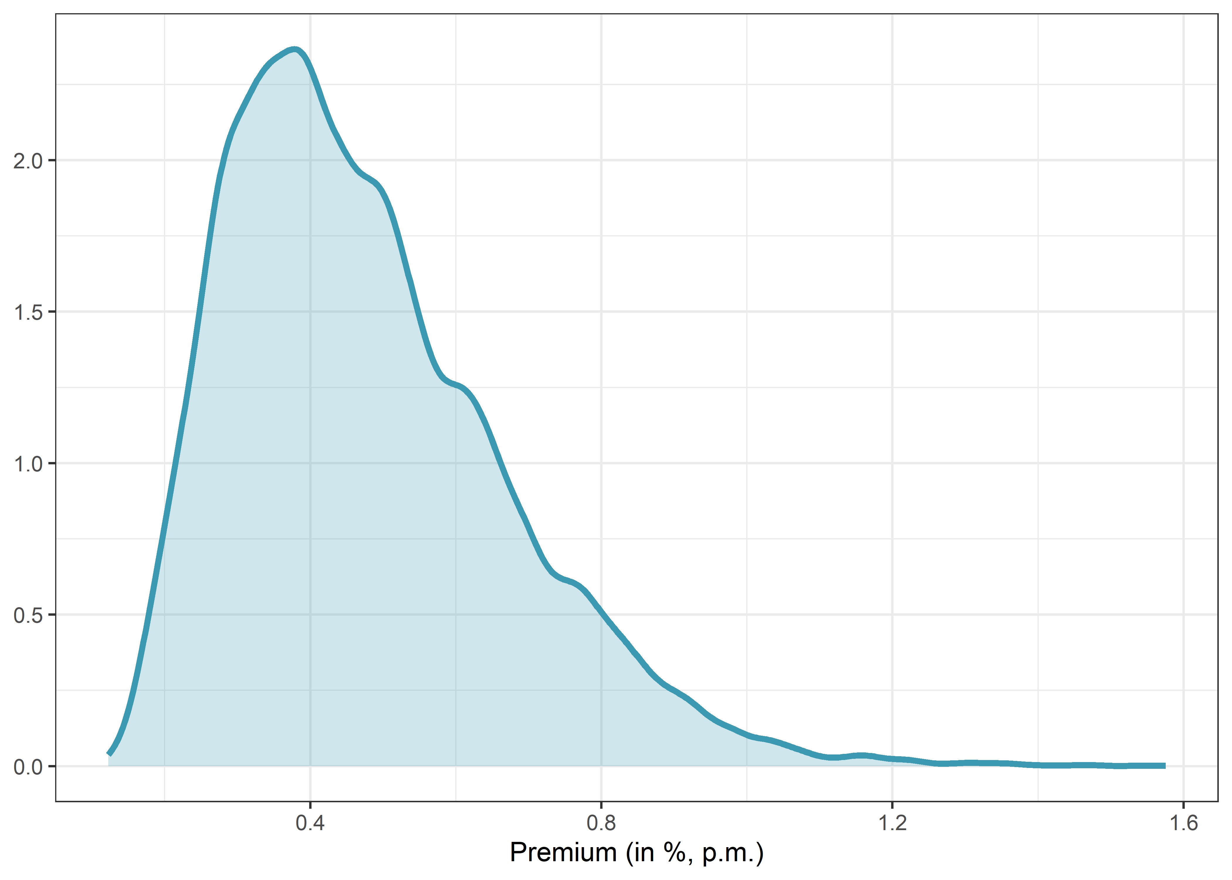
You can immediately see one of the results in Walter, Weber, and Weiss (2023): There is a lot of variation depending on your choices. However, despite the variation, the premium is always positive. I would argue that this is a pretty strong sign.
Conclusion
In summary, there are many potential ways of sorting the cross-section of stocks into portfolios. We explored 69,120 different possibilities based on decisions taken in published research articles. These choices induce variation that we embrace by considering all the possible paths.
In practice, most research papers introducing a new predictor usually present one of the specifications we have explored here, followed by a few robustness checks. These checks are commonly limited by space constraints. However, our analysis could be viewed as nearly 70,000 robustness tests condensed into an easily interpretable graph or two (if we include t-statistics). Personally, I find this approach both compelling and efficient.
Naturally, we still have to scrutinize the time series of return differentials against a factor model to demonstrate that existing factors cannot capture the suggested premium. I did not include this step in our discussion as it is a straightforward extension of the code we have used. I encourage you to give it a try.
For those interested in delving deeper into non-standard errors in portfolio sorts, I recommend reading Walter, Weber, and Weiss (2023). It provides a comprehensive overview of numerous variables and a more profound analysis of the variation itself.
Footnotes
Menkveld, A. J. et al. (2023). “Non-standard Errors”, Journal of Finance (forthcoming). http://dx.doi.org/10.2139/ssrn.3961574↩︎
Walter, D., Weber, R., and Weiss, P. (2023). “Non-Standard Errors in Portfolio Sorts”. http://dx.doi.org/10.2139/ssrn.4164117↩︎
Cooper, M. J., Gulen, H., and Schill, M. J. (2008). “Asset growth and the cross‐section of stock returns”, The Journal of Finance, 63(4), 1609-1651.↩︎