Tidy Finance - CIR Model Calibration using Python

The Cox–Ingersoll–Ross (CIR)¹ model stands as a cornerstone within the vast expanse of Financial Mathematics literature. Originally conceived to refine the well-known Vasicek² model in Interest Rate Modeling, the CIR model addressed a notable limitation of its predecessor—specifically, the propensity of Gaussian models like Vasicek’s to generate negative interest rates, a feature often deemed undesirable despite the theoretical possibility of negative rates in reality.

In this concise exposition, I will delineate the process of calibrating the Cox–Ingersoll–Ross model using Python. From a theoretical point of view, I will define linear models to calibrate the CIR model and test their feasibility via Monte-Carlo simulations.

CIR Model - Overview

The CIR model aims to capture the dynamics of interest rates, offering a powerful alternative to the Vasicek model.

The Vasicek model can be mathematically defined by an Ornstein–Uhlenbeck process with an added drift term. This is a stochastic process particularly suitable for interest rate dynamics, owing to its inherent properties of stationarity and mean-reversion. These attributes align with the behavior commonly observed in interest rates.

The SDE (stochastic differential equation) for the Vasicek model is the following (where \(dW_t\) denotes the Wiener process): \[ dr_t=k(\theta-r_t)dt+\sigma dW_t \]

Moreover, the model yields an intuitive interpretation of its parameters:

\(\theta\) is the long-run average
\(k\) is the intensity with which the process returns to its long-run average
\(\sigma\) is the instantaneous volatility

In contrast, the CIR model differs by introducing a novel component into the diffusion part of the process, precisely \(\sqrt{r_t}\), as depicted below: \[ dr_t=k(\theta-r_t)dt+\sigma\sqrt{r_t}dW_t \]

This seemingly minor adjustment has profound implications, as it ensures that interest rates remain strictly positive. However, this modification also engenders notable distinctions between the two models.

Without delving into mathematical intricacies, it is imperative to recognize that while the Vasicek model adheres to a Gaussian process, the CIR model deviates from this, leading to a substantially more intricate conditional distribution. However, it is not necessary to grasp the intricacies of the distribution to develop Ordinary Least Squares (OLS) estimates, as elucidated in this article.

Model Discretization

The initial step necessitates discretization to manage the CIR model effectively and derive OLS estimates. This task is efficiently achieved through the Euler-Maruyama Scheme, a numerical method enabling the transformation of the stochastic differential equation (SDE) into a discrete-time equation. Essentially, this scheme involves approximating each differential term as a finite difference, with the accuracy of the approximation improving as the time step decreases.

This leads to the following equation: \[ r_{t + \delta t} - r_t = k(\theta - r_t)\delta t + \sigma \sqrt{r_t}N(0, \delta t) \]

Following some straightforward manipulations, it can be rewritten as: \[ \frac{{r_{t + \delta t} - r_t}}{{\sqrt{r_t}}} = \frac{k\theta \delta t}{\sqrt{r_t}} - k\sqrt{r_t} \delta t + \sigma \sqrt{\delta t} N(0,1) \]

This can be interpreted as: \[ y_i = \beta_1 z_{1,i} + \beta_2 z_{2,i} + \epsilon_i \]

Where: \[ \begin{aligned} y_i &= \frac{r_{t+\delta t}-r_t}{\sqrt{r_t}} \\ \beta_1 &= k\theta \\ \beta_2 &= -k \\ z_{1,i} &= \frac{\delta t}{\sqrt{r_t}} \\ z_{2,i} &= \sqrt{r_t}\delta t \\ \epsilon_i &= \sigma \sqrt{\delta t} N(0,1) \end{aligned} \]

Estimating the parameters of interest then becomes straightforward: \[ \begin{aligned} \hat{k} &= -\hat{\beta_2} \\ \hat{\theta} &= \frac{\hat{\beta_1}}{\hat{k}} \\ \hat{\sigma^2} &= \frac{\hat{Var(\epsilon)}}{\delta_t} \end{aligned} \]

Python Implementation

Upon reviewing the mathematical details, the next step is to translate them into Python code. I will define two functions:

simulate_cir(): This function simulates a path based on theoretical parameters. It is important to note that in the CIR model, the term \(\sqrt{r_t}\) requires that \(r_t\) remains non-negative. However, since we are working with a discrete form of the model, simulation errors may arise due to negative rates stemming from the random component of the model. These errors need to be addressed. This is facilitated by the following piece of code: np.sqrt(max(0, r)), which guarantees that no negative interest rate is passed under the square root.
ols_cir(): This function performs the estimates based on a given array of values.

# import libraries
import numpy as np
from sklearn.linear_model import LinearRegression
import matplotlib.pyplot as plt
import seaborn as sns

# function to simulate paths
def simulate_cir(k, theta, sigma, r0, T, N):

    # populate an empty array
    dt = T / N
    interest_rate_paths = np.zeros(N+1)
    interest_rate_paths[0] = r0 
    for t in range(1, N+1):
        Z = np.random.randn()
        r = interest_rate_paths[t-1]
        interest_rate_paths[t] = r + k * (theta-r) * dt + sigma * np.sqrt(dt) * np.sqrt(max(0, r)) * Z    
    return interest_rate_paths

# function to estimate parameters
def ols_cir(data, dt):

    # define variables
    Nsteps = len(data)
    rs = data[:Nsteps - 1]  
    rt = data[1:Nsteps]
    
    # model initialization
    model = LinearRegression()

    # feature engineering to fit the theoretical model
    y = (rt - rs) / np.sqrt(rs)
    z1 = dt / np.sqrt(rs)
    z2 = dt * np.sqrt(rs)
    X = np.column_stack((z1, z2))

    # fit the model
    model = LinearRegression(fit_intercept=False)
    model.fit(X, y)

    # calculate the predicted values (y_hat), residuals and the parameters
    y_hat = model.predict(X)
    residuals = y - y_hat
    beta1 = model.coef_[0]        
    beta2 = model.coef_[1]

    # get the parameter of interest for CIR
    k0 = -beta2
    theta0 = beta1/k0
    sigma0 = np.std(residuals)/np.sqrt(dt)
    
    return k0, theta0, sigma0

The subsequent step involves applying these functions to a specific case by fixing theoretical parameters for the CIR model. In this instance, I will opt for relatively standard parameter values. However, a more formal analysis would require exploring a range of values for each parameter to evaluate the robustness of the estimators under different conditions.

k_true = 5 # True mean reversion speed
theta_true = 0.05  # True long-run mean
sigma_true = 0.03 # True volatility of interest rates
r0_true = 0.3 # True initial interest rate
T = 1  # Time horizon
N = 100  # Number of time steps
dt = T/N

# simulated path
np.random.seed(123)
series = simulate_cir(k_true, theta_true, sigma_true, r0_true, T, N)
estimates = ols_cir(series, dt)

# print results
print(f"The theoretical parameters are: k={k_true}, theta={theta_true}, sigma={sigma_true}")
print(f"The estimates are: k={round(estimates[0], 3)}, theta={round(estimates[1], 3)}, sigma={round(estimates[2], 3)}")

The theoretical parameters are: k=5, theta=0.05, sigma=0.03
The estimates are: k=5.078, theta=0.051, sigma=0.034

Monte-Carlo Results

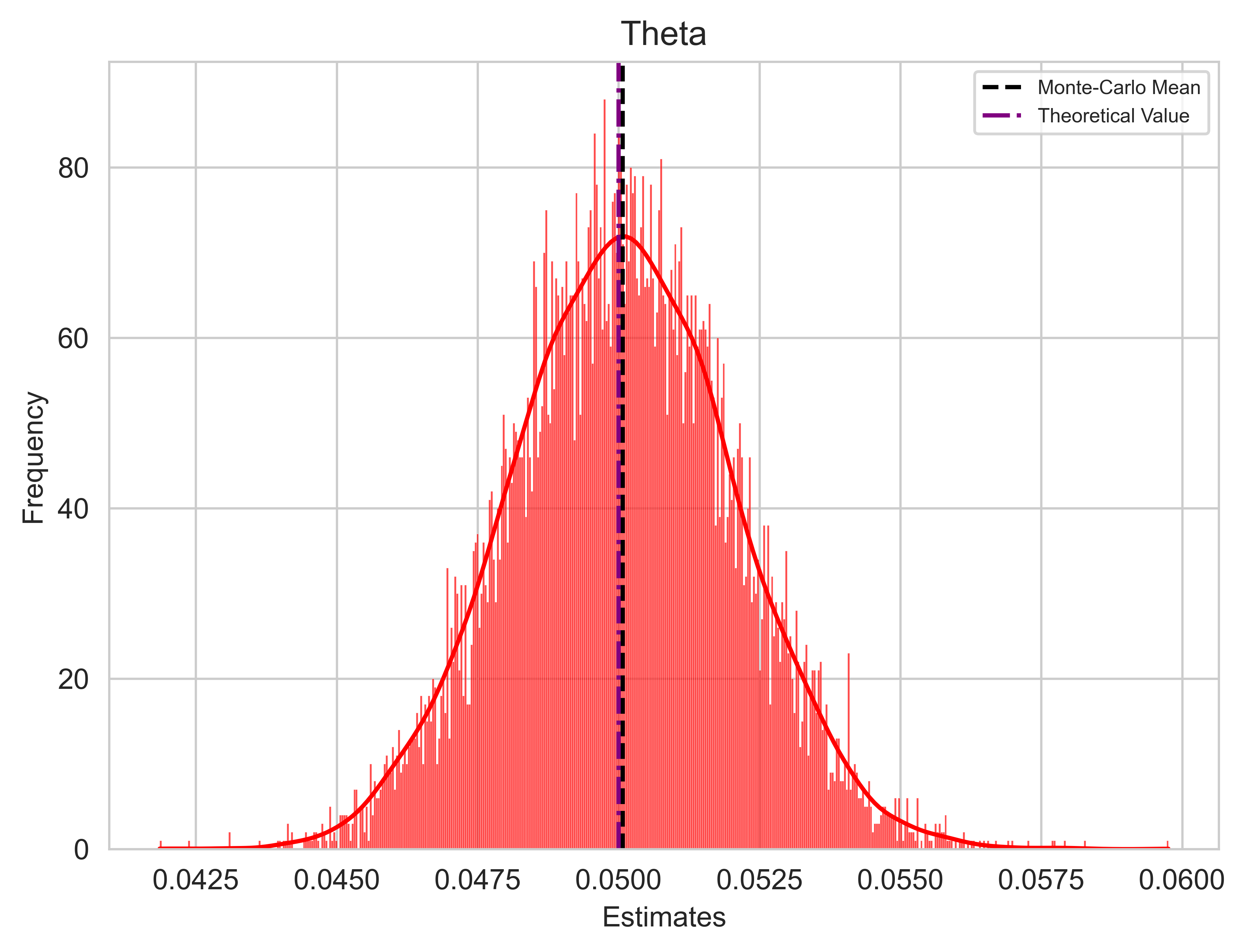
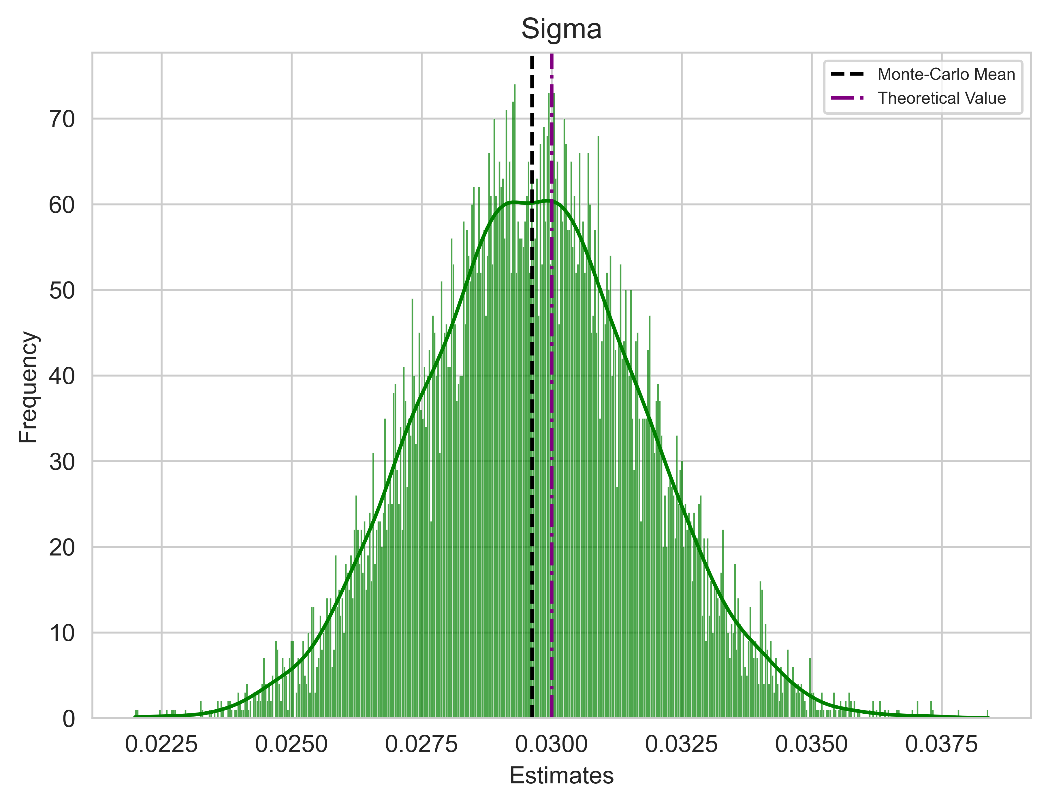
The final step entails conducting a Monte Carlo Simulation to thoroughly scrutinize how the estimators perform. The model comprises two components: a deterministic one and a stochastic one. In the preceding step, I calibrated the model using a single vector of Gaussian samples, which generated a particular path. Now, I will repeat this process with several different vectors of Gaussian samples, generating multiple paths while maintaining the same real parameters.

If the estimators are reasonably accurate, we should observe a convergence of the Monte Carlo estimates means towards the real parameters, indicating the unbiasedness of the estimators in principle.

It is important to note that due to discretization errors, there is a possibility of generating paths with negative interest rates. To address this issue, I will adopt the approach suggested in Orlando, Mininni, and Bufalo (2020)³, which involves shifting all series by the 99th percentile before the calibration. This allows, in most cases, to work with a positive series of data. It is crucial to highlight that if we intend to use the calibrated model for predictions, we must subsequently subtract the same quantity from the predictions. This adjustment is implemented in the code via an if statement within the while loop.

# define variables
n_scenarios = 10000
paths = np.zeros(shape=(n_scenarios, N+1))
OLS_estimates = np.zeros(shape=(n_scenarios,3))

# perform simulations
np.random.seed(123)
count = 0
while count < n_scenarios:
    # fill the array with the simulations
    series = simulate_cir(k_true, theta_true, sigma_true, r0_true, T, N)
    
    # Check if there's at least one negative number in the series
    if np.any(series < 0):
        # Calculate the value of the 99th percentile
        percentile_99 = np.percentile(series, 99)
        # Add the value of the 99th percentile to each element of the series
        series += percentile_99

    paths[count, :] = series
    
    # OLS estimation
    estimates = ols_cir(series, dt)
    OLS_estimates[count,:] = estimates
    
    # update counter
    count += 1

# plot of the estimates distributions
colours = ["blue", "red", "green"] 
parameters = ["k", "Theta", "Sigma"] 
real_values = [k_true, theta_true, sigma_true]

# Set the seaborn style
sns.set_style("whitegrid")
for i in range(3):  # Using range(3) for iterating over indices

    # Set up the plot
    plt.figure(figsize=(7, 5))
    sns.histplot(OLS_estimates[:, i], bins=500, color=colours[i], alpha=0.7, kde=True)

    # Plot mean as black dot line
    mean_estimate = np.mean(OLS_estimates[:, i])
    plt.axvline(mean_estimate, color="black", linestyle="--", label="Monte-Carlo Mean")

    # Plot specified value as purple dot line
    plt.axvline(real_values[i], color="purple", linestyle="-.", label="Theoretical Value")

    plt.xlabel("Estimates", fontsize="medium")
    plt.ylabel("Frequency", fontsize="medium")
    plt.title(parameters[i], fontsize="large")
    plt.legend(title_fontsize="small", fontsize="x-small")
    plt.show()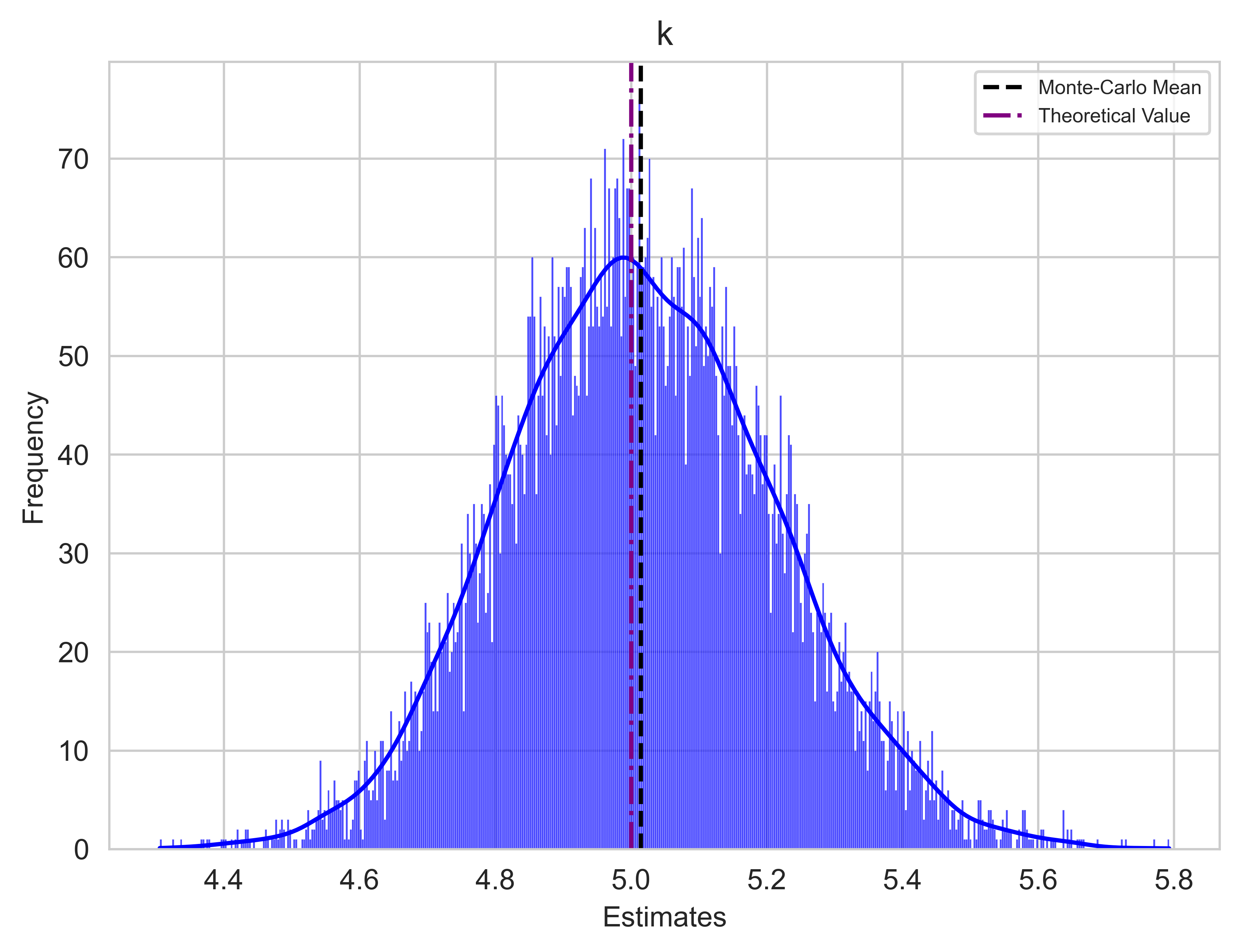

Figure 1: Results of Monte Carlo Simulation for parameter k.

Figure 2: Results of Monte Carlo Simulation for parameter Theta.

Figure 3: Results of Monte Carlo Simulation for parameter Sigma.

Conclusions and Real-World Application

To summarise, this article has covered:

Introduction to the CIR model
Implementation of OLS estimators for model calibration
Evaluation of estimator performance via Monte Carlo simulations

To conclude, let’s include a final snippet code to apply the routine to real-world data. I will fetch the 13-week Treasury Bill Rate using the yfinance package and then apply the ols_cir function to calibrate the model. Here are a couple of insights on the code:

Data covers all of 2023
Following convention, dt is set to 1/252 since there are approximately 252 trading days in a year, and interest rates are expressed in annual terms

import yfinance as yf

# Ticker symbol for US interest rate
ticker_symbol = "^IRX"  # 13 Week Treasury Bill Rate

# Fetch data
interest_rate_data = yf.download(ticker_symbol, start="2023-01-01", end="2024-01-01")
interest_rate_data = interest_rate_data["Close"]/100 # divide by 100 as the data are expressed in percentage
dt = 1/252

# model calibration
estimates = ols_cir(interest_rate_data.values, dt)
print(f"The estimates are: k={round(estimates[0], 3)}, theta={round(estimates[1], 3)}, sigma={round(estimates[2], 3)}")

[*********************100%%**********************]  1 of 1 completed
The estimates are: k=6.442, theta=0.052, sigma=0.03

Footnotes

Cox, J. C., Ingersoll Jr, J. E., & Ross, S. A. (1985). A Theory of the Term Structure of Interest Rates. Econometrica, 53(2), 385-408. Link.↩︎
Vasicek, O. (1977). An equilibrium characterization of the term structure. Journal of financial economics, 5(2), 177-188. Link.↩︎
Orlando, G., Mininni, R. M., and Bufalo, M. (2020). Forecasting interest rates through vasicek and cir models: A partitioning approach. Journal of Forecasting, 39(4):569–579. Link.↩︎